Tutorial 1: NGS Pipeline with Custom Interactive Selection (PacBio), In-Vitro Library

Background

A selection campaign using a semi-synthetic, codon-optimized, antibody library was carried out against the SARS-COV-2 antigen Spike(S) trimer and its subunit S1 and the S1 subunit RBD. Three independent selection campaigns were carried out using the same input library. DNA was isolated from a less stringent population, 2 rounds of in-vitro selection at 10nM, and a more stringent population, 3 rounds of in-vitro selection at 1nM. Each population was prepared by PCR amplification with the addition of in-line barcode consisting of 8mer (DNA) barcodes at the 5’ and 3’ ends to distinguish the 6 populations consisting of:

1) 2 x trimer (early and late rounds)

2) 2 x S1 (early and late rounds)

3) 2 x RBD (early and late rounds)

All input files can be located in Orion in following location:

Organization Data / OpenEye Data / Tutorial Data / AbXtract /

A barcode table titled ‘barcode_file_abxtract.xlsx’ indicates how these samples were prepared. Amplified DNA products were pooled together in a single tube and shipped to a PacBio / Illumina sequencing provider. The provider then shipped us back one PacBio file titled ‘pacbio_small_codon_optimized.fastq’ and two illumina files titled ‘F_illumina_codon_optimized_abxtract.fastq and R_illumina_codon_optimized_abxtract.fastq’, respectively. The PacBio file consists of a set of sequences each of length ~800bp composed of variable light (VL) and variable heavy (VH) sequences in VL-linker-VH orientation. The Illumina files consist of one forward and one reverse FASTQ file. Each sequence within the FASTQ is ~300bp in length, with an overlapping region between the forward and reverse reads to enable paired end assembly of the sequences into one VH sequence.

For the purposes of this tutorial, each of the FASTQ files from PacBio/Illumina was reduced by taking a random output of 87,966 sequences for PacBio and 84,988 sequences from Illumina. The larger files from which these were derived contain an underlying diversity of full-length nucleotide of ~50k total, with a 20-fold reduction in the H3 diversity.

All populations are derived from the same input library against three overlapping subunits of the Spike (S) protein. The goal of this tutorial is to cluster all three populations binding to the Spike (S) trimer, which encompasses S1. S1 can further be broken into smaller units, one of which is the receptor binding domain (RBD). Because each domain is subunit of the other, we anticipate overlap among RBD, S1 and trimer, particularly since the same input library was used during this selection. We anticipate we will also find antibodies that are unique to select subunits (e.g. S1 only), likely due to 1) non-overlapping regions (e.g., epitopes on trimer outside of S1), 2) exposed regions that are available in recombinant form but not in complex (e.g., S1 in trimer complex versus S1 in recombinant form), 3) and conformational changes from native or complex form versus recombinant form.

The goal of the tutorial is to identify overlapping regions of interest (ROI) particularly at the heavy chain complementarity determining region (HCDR3), which is most often implicated in binding specificity of the antibody to the target. In particular, we will use the HCDR3 to identify the output populations that overlap across the RBD, S1 and trimer populations as we hypothesize the population at the intersection are likely to exhibit optimal binding profiles in the native conformation of the RBD in vivo, which will result in more optimal neutralization (RBD) potential relative to those HCDR3s that only recognize recombinant versions of the RBD or S1. Further, we want to ensure that antibodies display more favorable NGS metrics (high relative abundance, elevated fold enrichment, increased copy number of the full-length antibody, and reduced number of liabilities that may present problems during scaling up processes).

STEP 1 - Login to Orion, Set-Up Directory, Locate Tutorial Files

1. If the sequencing provider provides FASTQ files that are compressed (e.g., ends with “.gz” or “.zip”), decompress with a standard decompressor so the file ends with .fastq. If any suffix is added to the end, make sure to modify these suffixes so they end in .fastq for all sequence files to be processed.

2. Log into the Orion interface with your email and password. Find the 3 required files under Organization Data as follows:

   A) Organization Data / OpenEye Data / Tutorial Data / AbXtract / pacbio_small_codon_optimized.fastq

   B) Organization Data / OpenEye Data / Tutorial Data / AbXtract / barcode_file_abxtract.xlsx

   C) Organization Data / OpenEye Data / Tutorial Data / AbXtract / scaffold_ref_db_codon_optimized_dna.txt

3. Create a general tutorial directory and tutorial 1 subdirectory under PROJECT DIRECTORY / TUTORIALS / TUTORIAL_1 (This is your BASE DIRECTORY and should be used for all outputs for this Tutorial 1 below).

STEP 2 - Select the ‘NGS Pipeline’ Floe

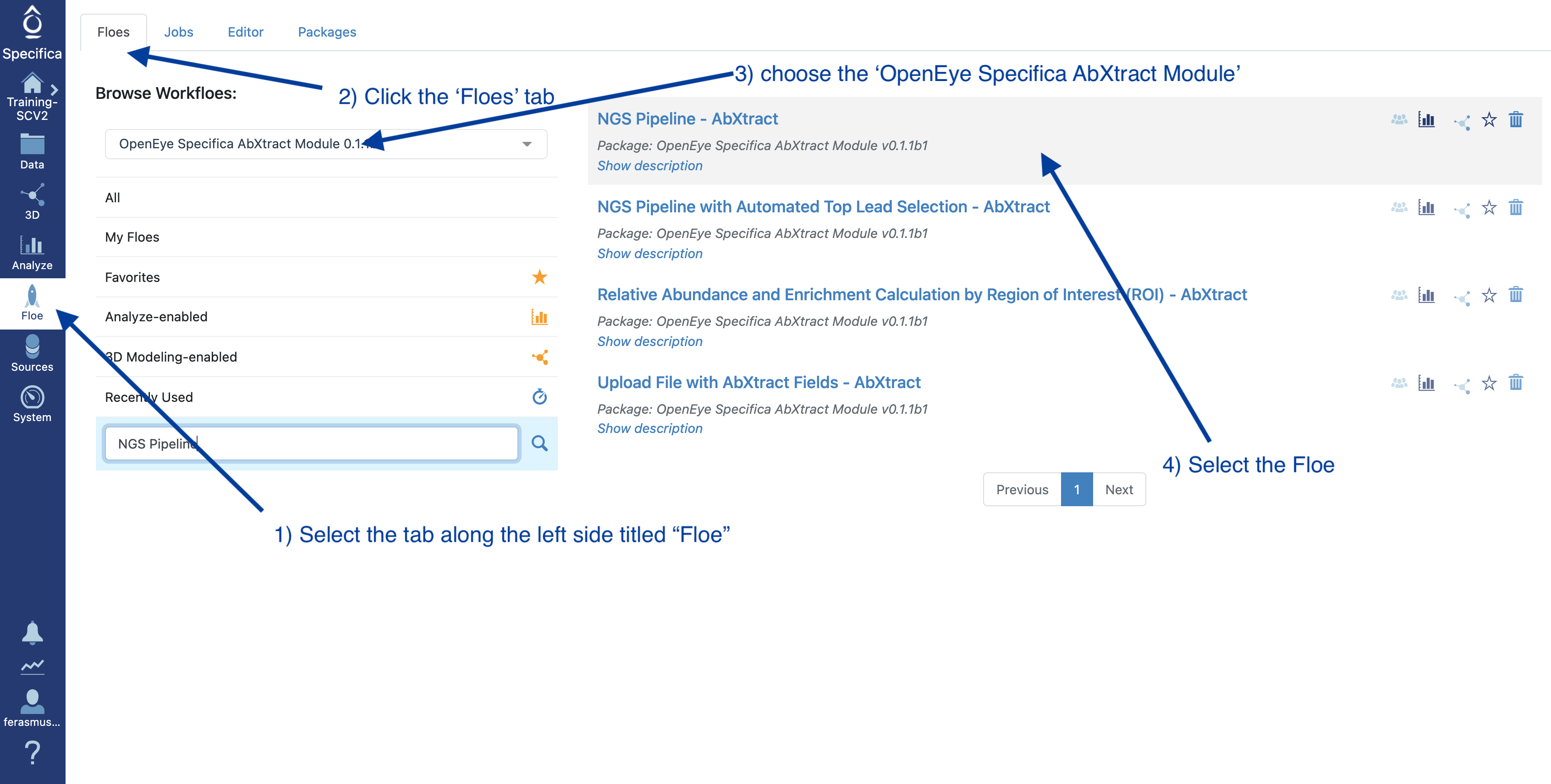
1. Select the tab along the left side tab titled ‘Floe’.

2. Click the ‘Floes’ tab.

3. Choose the ‘OpenEye Specifica AbXtract Module’.

4. Select the Floe ‘NGS Pipeline’.

STEP 3 - Prepare PacBio Run and Start Job

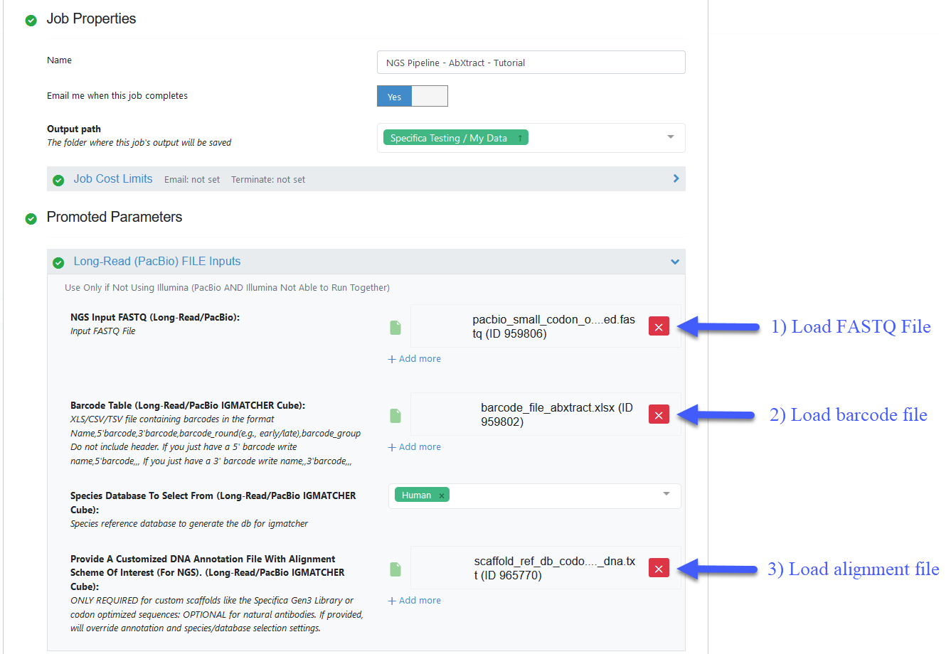
1. Load FASTQ file - ‘pacbio_small_codon_optimized.fastq’.

2. Load barcode XLSX file - Organization Data / OpenEye Data / Tutorial Data / AbXtract / ‘barcode_file_abxtract.xlsx’.

3. Load alignment TXT file - Organization Data / OpenEye Data / Tutorial Data / AbXtract / ‘scaffold_ref_db_codon_optimized_dna.txt’.

Important Note

All the remaining parameters can be kept as the default values. Scroll through remaining “Promoted” parameters to get a sense of these parameters.

4. Click ‘Start Job’.

STEP 4 - Open the Floe Report to Get a General Idea About the Population

1. Under the ‘Jobs’ tab find the ‘NGS Pipeline’.

2. Click the ‘Show non-dataset files’ checkbox. The breakdown of datasets, collections (Floe reports) and files (CSV) are depicted here:

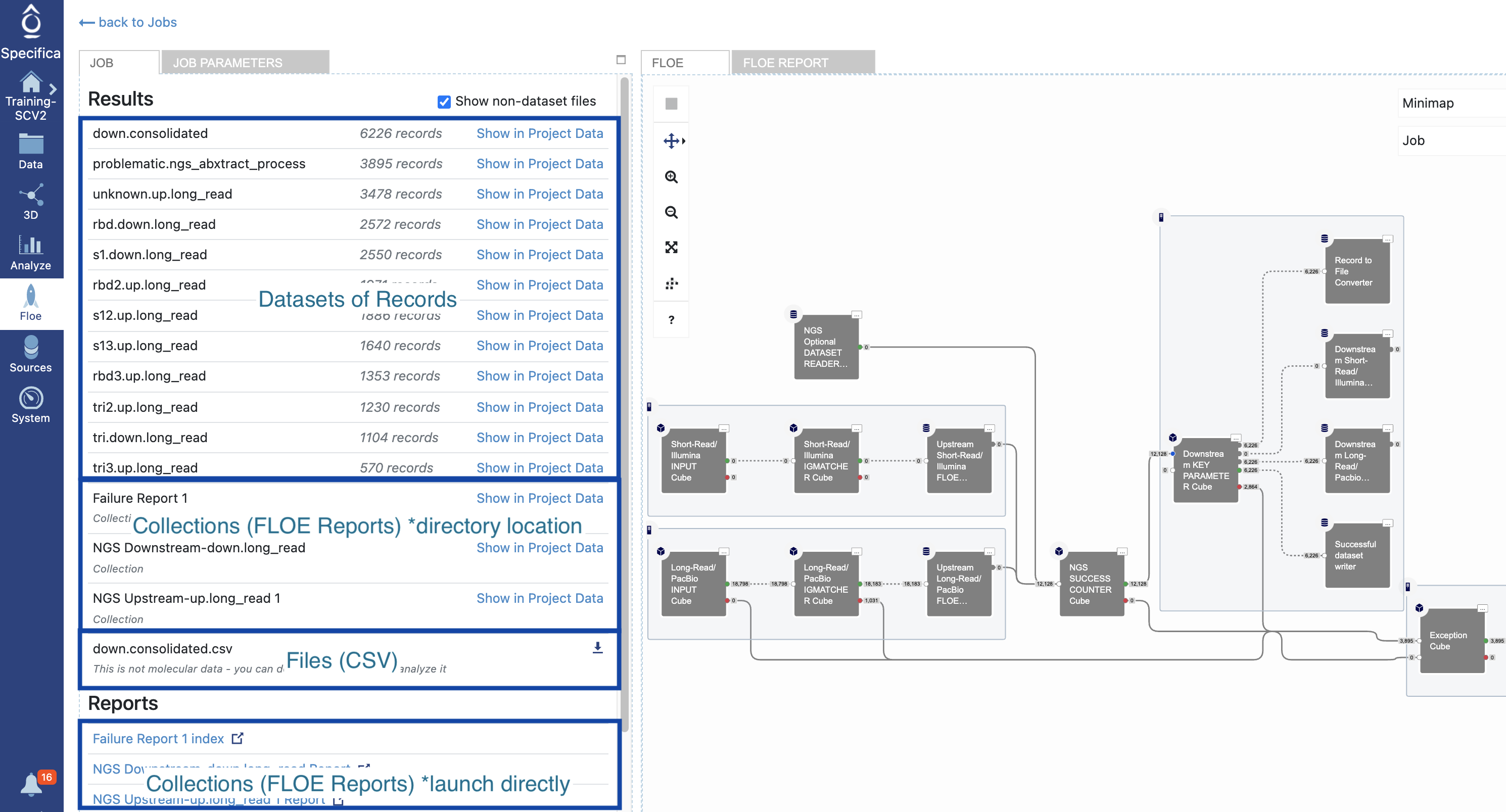
3. Click on the ‘NGS Downstream-down.long_read’ under the ‘Reports’ section to launch in browser. Give it some time to load in browser.

4. See the ‘General stats’, which provides a snapshot of the number of non-redundant full-length, LCDR3, HCDR3, LCDR3 and HCDR3 sequences. Chain_1 represents the variable light chain (VL) and chain_2 represents the variable heavy chain (VH). The overlap shows the overlap of the region of interest (HCDR3) across the different populations.

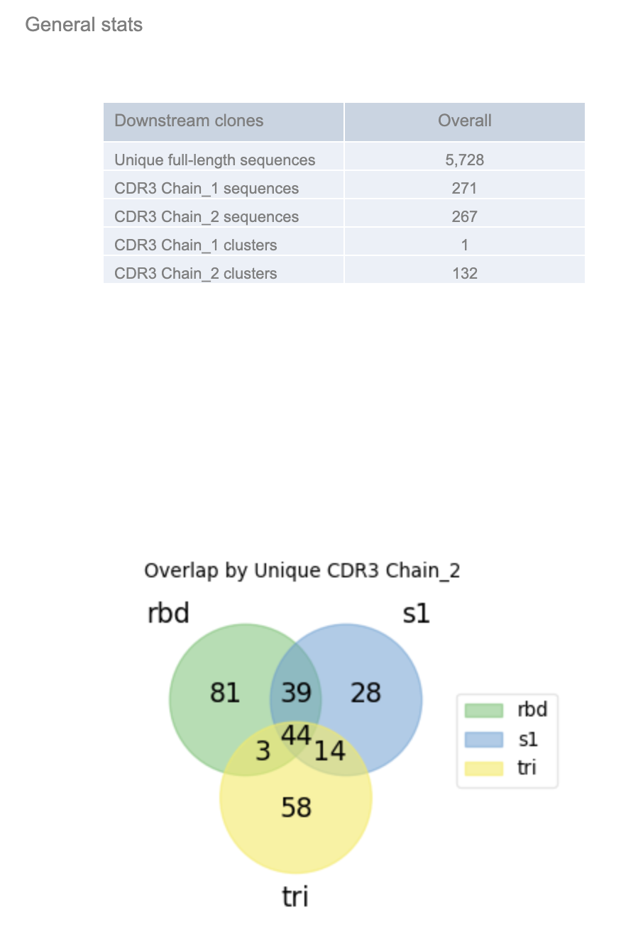
5. Each subpanel separates out the ‘barcode_group’ and shows the population specific (e.g., trimer, S1, RBD) statistics.

6. Return to Job overview of all the datasets, floe reports and files - see above.

7. Find the dataset called ‘down.consolidated’ and click ‘Show in Project Data’:

STEP 5 - Activate the Dataset

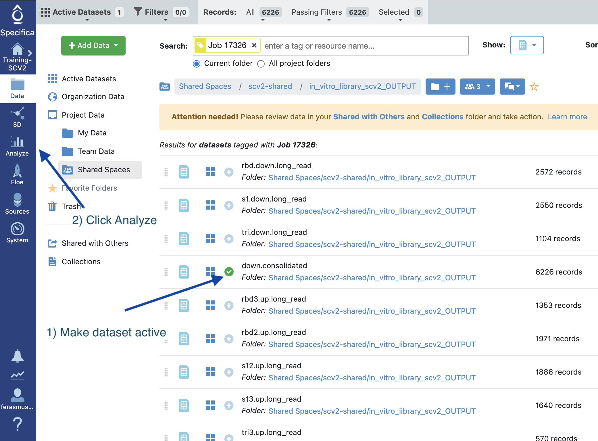
1. Select the ‘+’ symbol next to the dataset called ‘down.consolidated’.

2. Select the Analyze tab.

STEP 6 - Plot Relative Abundance Versus Desired Overlap Population and Select Population with Analyze Tool

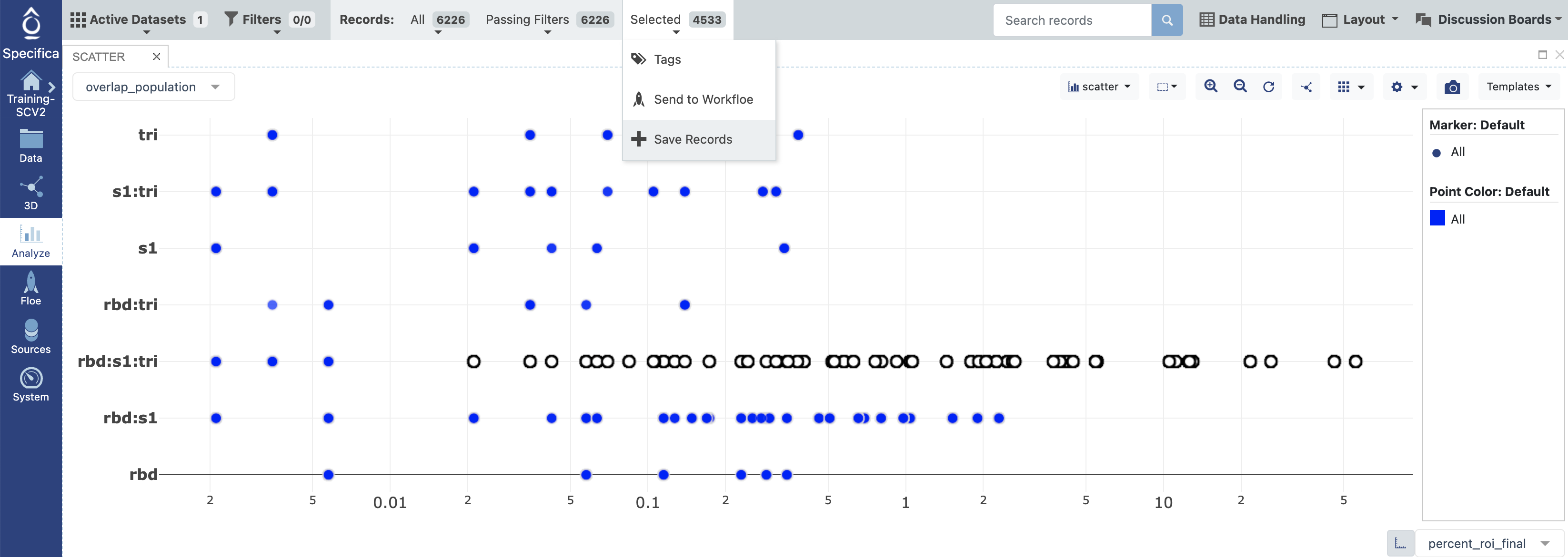
1. Select x-axis: percent_roi_final.

2. Select y-axis: overlap_population.

3. Subselect records within the rbd:s1:trimer population with an ROI above the 0.01% as shown above.

4. At top of the interface next to the ‘Selected’ tab it should state the amount of selected antibodies, click on this and choose the option (+ Save Records).

5. Click the button called “New Dataset”, name the new dataset “rbd_s1_trimer>0.01”, select the option ‘Do nothing’ and choose the BASE DIRECTORY see STEP 1, #3.

6. Allow some time for it to generate the new dataset, ~4.5k records. Find the new dataset in directory that was specified. The dataset may be grayed out indicating it needs additional time to process. If after time it is still grayed out, select the ‘…’ ellipses to right of dataset and choose ‘Process Data’ option.

7. Make sure to remove any active datasets by selecting the ‘Active Datasets’ dropdown near the top left and select ‘Clear All’.

STEP 7 - Select the Enriched Population Using the Analyze Tool and Send to Automated Top Lead Selection Floe

1. Make the newly created dataset ‘rbd_s1_trimer>0.01’ active.

2. Find the ‘Data Handling’ option bar near the top right.

3. Make sure that the log2_enrichmment_roi is active across ‘All’. Select ‘Apply’.

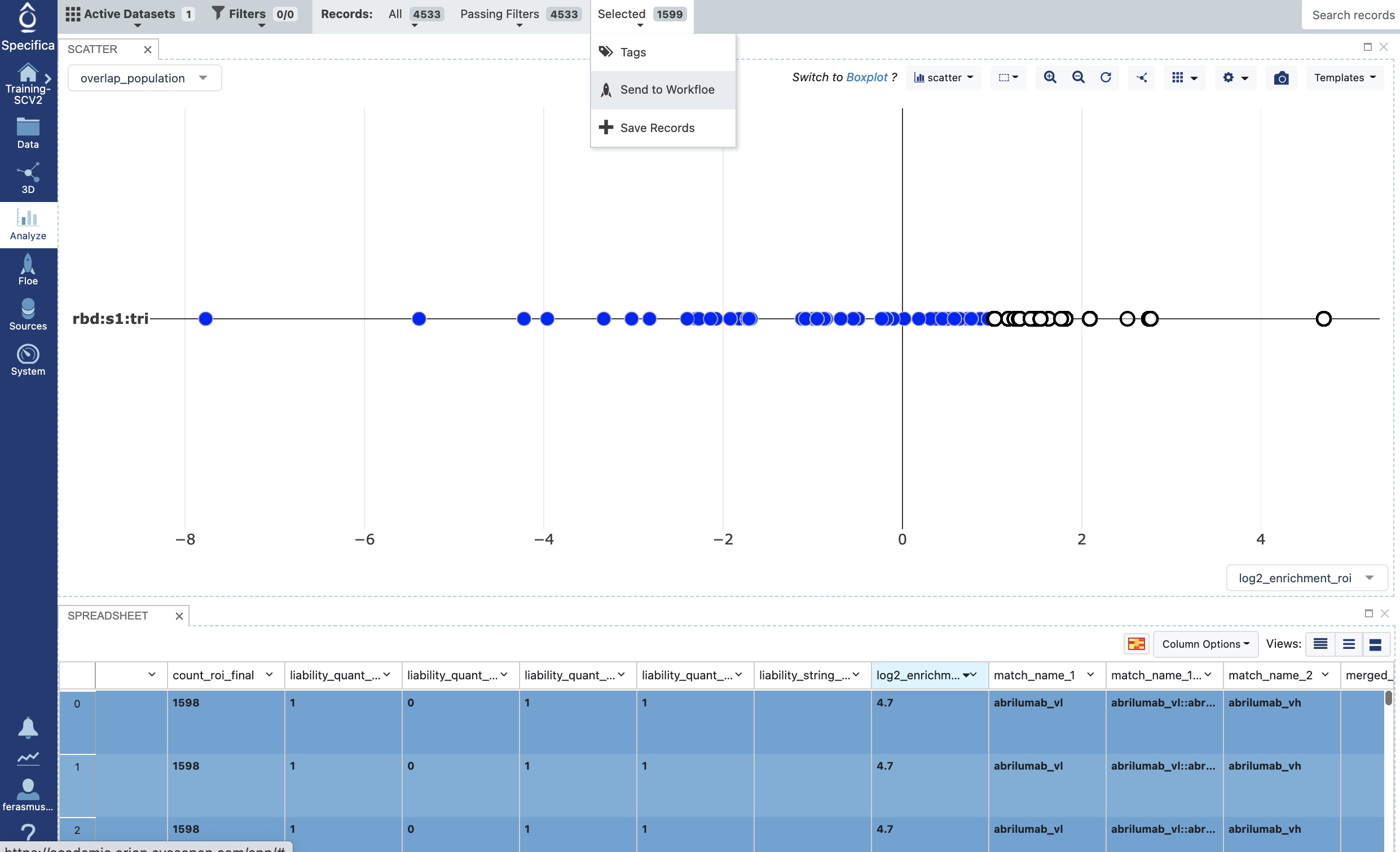
4. On x-axis, select the ‘log2_enrichment_roi’ option. If it doesn’t appear in initial display screen, use default x-axis and y-axis, then immediately click cancel. log2_enrichment should appear in dropdown menu for x-axis parameters. For y-axis choose any parameter (e.g., overlap_population).

5. Choose records with log2_enrichment of ≥ 1 in the table. Find the field ‘log2_enrichment_roi’ in the table, select the down arrow, and click sort descending.

6. Shift select all rows above the ≥ 1 in the table, selected population should be selected in the plot seen in image below.

7. Choose the ‘Selected’ tab near the top and choose ‘Send to Workfloe’ as depicted in the image.

8. Search for Workfloe titled ‘Automated Top Lead Selection’ and click the sub-option ‘View all Workfloe options’.

9. Set the Output path BASE DIRECTORY (see STEP 1, #3).

10. Set the ‘NGS Key Selection Parameters’ as default.

DESCRIPTION OF KEY SELECTION PARAMETERS

Maximum Number Of Full-Length Sequences - The maximum number of full-length, non-redundant sequences to output.

Maximum Number Sequences per Cluster - The maximum number of unique full-length sequences per given cluster.

Maximum Number Of Clusters Preferred - The maximum number of clusters that we want to select from.

Metrics For Ranking - Metrics that determine how the sequences will be sorted in output.

Rank Sanger Clones First In Population - Keeps SANGER population (ranked by same metrics as ‘metrics for ranking’) at the top of the rank order. Only used if SANGER dataset/file provided.

Attempt To Fill The Desired Number Of Full-Length Sequences Quota - Attempts to fulfill the total number of sequences Maximum Number Of Full-Length Sequences by selecting additional full-length sequences from same clusters followed by selecting the remaining top ranked clones from different clusters.

13. Keep the default output names.

14. Start Job.

STEP 8 - Subset the Number of Fields for Output and Download CSV

1. Find the dataset called ‘picked.consolidated’ created in STEP 7 within the data directory or directly from job (click Show in Project Data) as shown here:

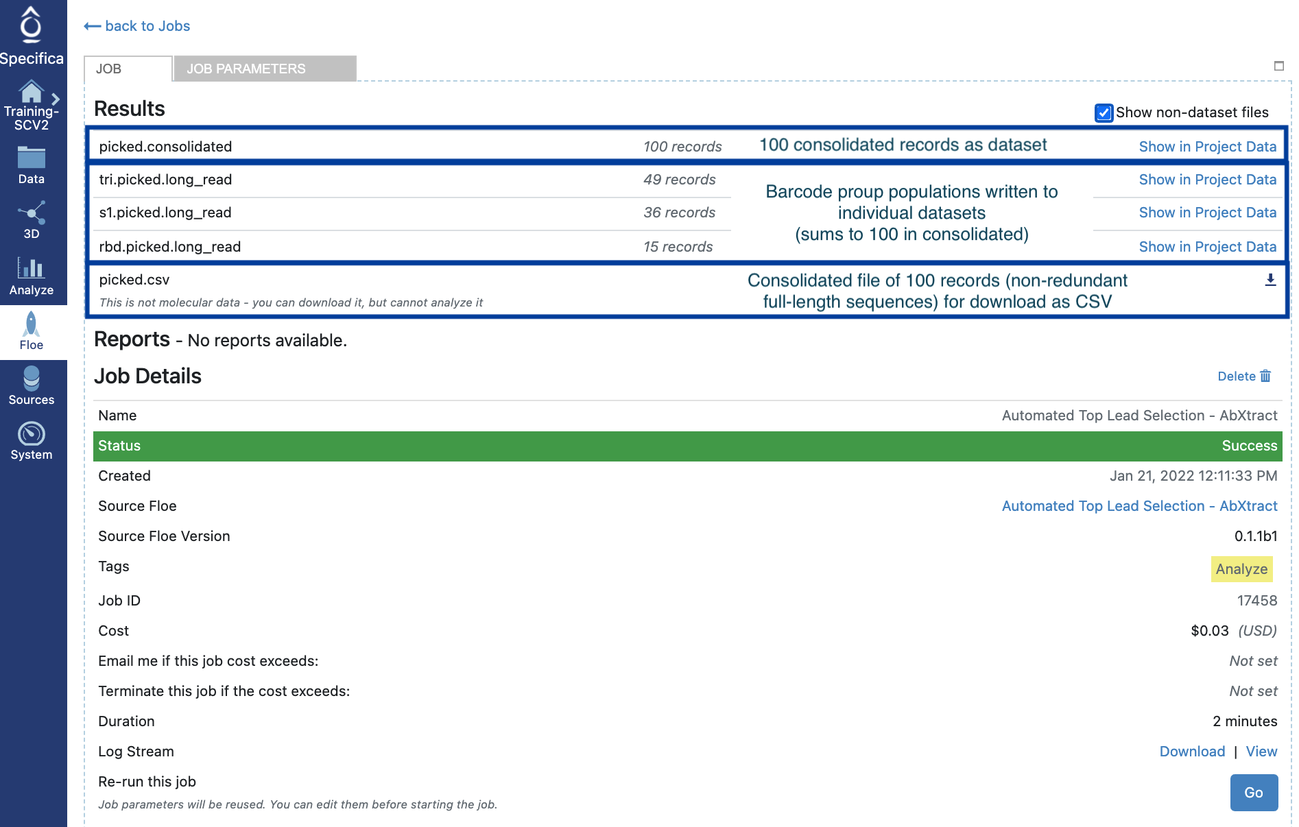
2. Find the symbol that states ‘Send to Workfloe’ to the right of the dataset title ‘picked.consolidated’ and find the Floe ‘Subset the Number of Fields for Export’ and ‘View all Workfloe Options’.

3. Keep following fields (for more details, see key fields reference):

   A) sequence_aa_1

   B) sequence_aa_2

   C) match_name_1

   D) match_name_2

   E) cluster

   F) seq_id

4. Give an output name:

   A) ‘gene_synthesis_clones_with_cluster_id’ for the output dataset.

   B) ‘gene_synthesis_clones_with_cluster_id.csv’ for the CSV file.

5. Click ‘Start Job’.

6. After completion, find the job associated with ‘Subset the Number of Fields for Export’. Open the job to view datasets, as follows:

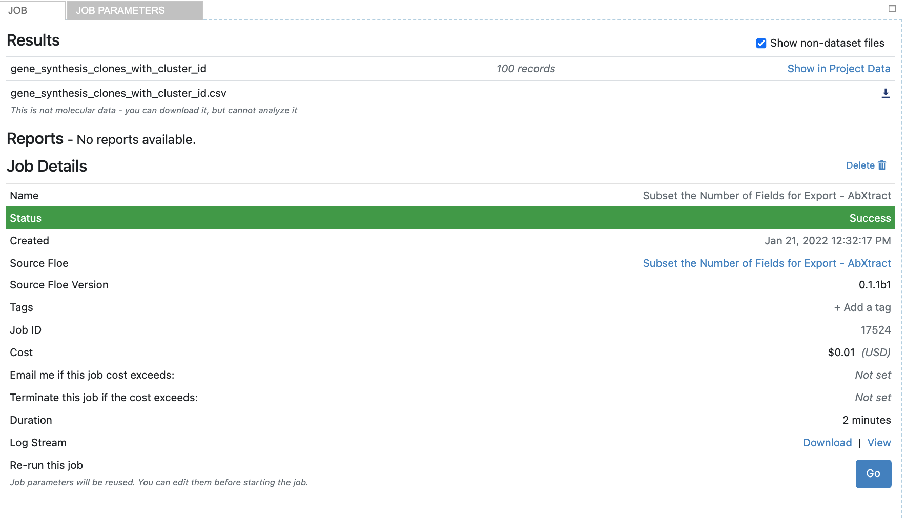
7. Click the checkbox titled ‘Show non-dataset files’ to find the CSV titled ‘gene_synthesis_clones_with_cluster_id.csv’.

8. Click the download to obtain the CSV list of sequences ready for gene synthesis.