Getting Started¶

This chapter provides a quick overview of AFITT and how to set it up to solve ligand structures for crystallography.

AFITT Workflows¶

AFITT is designed to support ligand fitting for common refinement workflows including REFMAC5,`Phenix.refine`, and CNS/X-Plor as well as providing automatic exporting of results to COOT or VIDA. These workflows are configurable at any time through a convenient dialog.

AFITT Supported Workflows¶

AFITT supports various workflows including using REFMAC and opening generated results in COOT. When AFITT is first opened, a welcome screen is displayed allowing the user to choose fom the available workflows as seen in Figure: Welcome To AFITT.

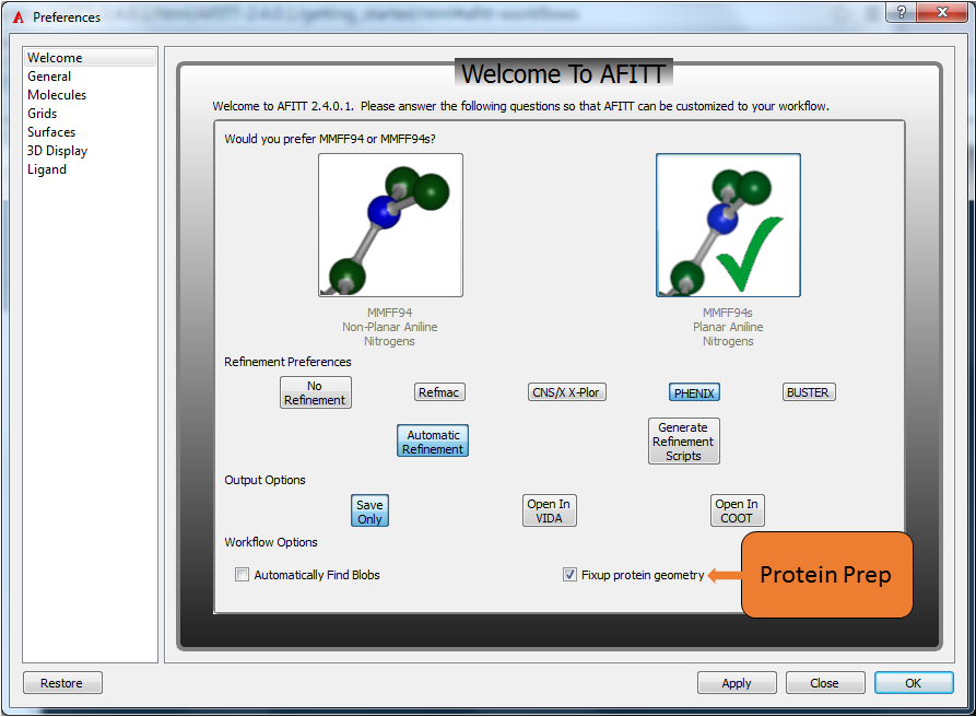
Welcome to AFITT

The tasks common to all workflows are:

Loading Molecules and Maps and identifying the ligand to fit.

Locating ligand density.

Fitting the ligand to the selected density.

At this point, if you are not doing a refinement, you can inspect the results and save them to disk. If desired, COOT or VIDA can automatically open the protein-ligand complexes.

If a refinement is being done, a dictionary file for the protein-ligand complex is generated along with the appropriate pdb and dictionary files for REFMAC5 or Phenix. REFMAC or Phenix.refine parameters can be changed or the REFMAC script can be edited before the refinement.

Once the refinement is completed, AFITT provides validation tools such as analyzing the real space correlation coefficient of the residues in the final structure and the ramachandran plot of the complex.

These workflows are summarized in figure Figure: AFITT Workflows.

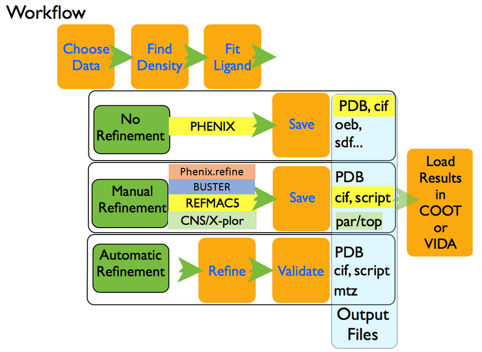
AFITT Workflows

MMFF Settings¶

AFITT supports the MMFF94 forcefield and it’s MMFF94s variant. The MMFF94s forcefield is a variant of MMFF94 that emulates time-averaged structures typically observed during crystallographic structure determination, mainly planar geometries at unstrained delocalized trigonal nitrogen centers. However, there are many theoretical studies that show puckering at nitrogen centers [Halgren-1999].

That being said, due to the prevalence of crystallographic studies, many chemists erroneously consider the time-averaged structure to be correct, hence this variant is available for use.

The implementation of AFITT’s MMFF forcefield is thorougly documented in the SZYBKI manual.

The MMFF setting can be adjusted in AFITT’s preferences window (see Figure: Welcome To AFITT) normally found under the File menu, or the AFITT menu if on OSX. Click on the image that has the desired nitrogen geometry and a green checkmark will appear indicating the current setting.

Select the planar aniline structure for MMFF94s or the puckered structure for MMFF94.

Hiding/Restoring Tips¶

To hide the tip window, simply click on the “Don’t show tips” checkbox in the tip dialog. To reenable tips used the Edit/Options menu and select Show Tips. Alternatively, open the preferences dialog and click on “Restore” to restore AFITT to the initial factory state.

How to Use AFITT¶

The AFITT interface is divided into a 3D scene on the right hand side, and a view of data relevant to the current task on the left. The basic overview of this is seen in Figure: Afitt Basic Overview:

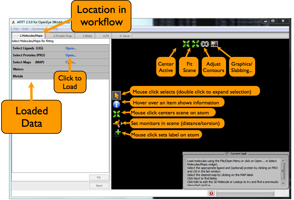
AFITT Basic Overview

3D Scene¶

There are two main components to using AFITT the most basic of which is interacting with the 3D scene. AFITT uses the same mouse modes as VIDA (although a COOT mouse mode is also available.) Please refer to Figure: AFITT Mouse Mode for more information.

AFITT Mouse Mode

Every 3D scene in AFITT has some basic capabilities, such as selecting items in the 3D scene; requesting further information such as residue and bfactor properties and setting distance and angle monitors. These secondary modes are toggled by selecting the appropriate icon from the 3D window as shown in figure Figure: Afitt Basic Overview.

Note

Use of these secondary modes is not required to run AFITT but can be useful during investigations of protein/ligand complexes. To quit a secondary mouse mode, click on the arrow icon.

Note

To change to the ‘COOT’ mouse mode, open up the preferences menu, navigate to the 3D Display menu and select “COOT” from the Mouse Map drop down menu. Note that selection in the 3D window will use the COOT conventions.

Common Operations¶

The toolbar at the top of the 3D Scene contains tools in common to manipulate the 3D scene. These tools include centering the current molecule to the screen center, fitting all visible objects to the scene, adjusting map contours, adjusting the depth cue and slabbing planes as well as turning stereo on and off. Stereo can also be turned on and off in the preferences dialog.

Selection¶

Objects in the display can be selected by clicking on them using the Left mouse button. The selection is cleared between button clicks (or by clicking in the background) unless the Shift or Ctrl key is also held down when clicking. If a single vertex on a surface has been selected, holding down the Shift key and selecting an second vertex will select the shortest path of vertices between the two selected end points.

Double-clicking using the Left mouse button expands the current selection to the next logical grouping. For instance, double-clicking on a selected atom in a protein will expand the selection to include all of the atoms in the same residue as the original selected atom. Double-clicking on the selected set again will expand the selection to include either the entire chain if there are multiple chains, otherwise it will include the entire molecule.

Selection can also be performed using a lasso style selection method by holding down the Right mouse button and moving the mouse in the window to define a selection rectangle (a dotted rectangle will be displayed on the screen as you do this). Releasing the Right mouse button will select all of the atoms and bonds inside of the rectangle. The previous selection will be cleared unless the Shift or Ctrl key is also held down while moving the mouse. Lasso style selection of surfaces and grids is not currently supported.

Rotation¶

The scene can be rotated in three dimensions by holding down the Left mouse button and moving the mouse in the window. These movements will emulate rotation using a trackball.

The scene can also be rotated around just the Z axis by holding down the Alt key and the Left mouse button simultaneously.

Translation¶

Using the mouse, the scene can be translated in the XY plane by holding down the Shift key and the Left mouse button simultaneously. Using the keyboard, the scene can be translated horizontally in the display by pressing either the A key or D key which translate to the left and to the right respectively.

Scale/Zoom¶

The scene can be scaled (or zoomed) by holding down the Middle mouse button by itself, the Left and Right mouse buttons together, or by using the mouse wheel. Any of these three modes will scale the scene. Multiple modes are provided for convenience and to accommodate the many varied mouse configurations in existence.

The scene can also be scaled using the W and S keys on the keyboard.

Text Scale¶

The scale of the text displayed in the scene can be controlled by using the mouse wheel while holding down the Ctrl key.

Clipping¶

The position of the near and far clipping (or slabbing) planes can be controlled using the mouse wheel while holding down both the Ctrl and Shift keys. Both planes are moved simultaneously and mirror each others’ positions. It is important to note that slabbing must already be enabled for these operations to actually be performed.

The clipping planes can be adjusted independently by holding down the Alt key with one of the Ctrl or Shift keys corresponding to the far and near clipping planes respectively.

Contour Level¶

The contour level of the active grids can be adjusted using the mouse wheel while simultaneously holding down the Shift key. Each incremental turn on the mouse wheel corresponds to an increase or decrease in the contour level by 0.1.

Label¶

Informative labels can be displayed about atoms and bonds (as well as surfaces and grid contours) underlying the current mouse position if the Ctrl key is pressed while moving the mouse (no mouse button need be depressed) on most platforms. On the Mac, this behavior is obtained by holding down the Alt key instead of the Ctrl key.

Wizard Operations¶

Most operations are completely automatic: loading and selecting the data to analyze and clicking Next are all that is normally required.

To load data, either use the Open command from the File menu or click on the appropriate Load button in the list window.

When the data is loaded, molecules are split into covalently bound regions and all loaded items are organized into Ligands, Proteins and Maps for easier access. To chose the data to operate on, simply select the ligand to fit by clicking on the LIG text in the list window. Select the proteins to use by clicking on the PRO text. Likewise, maps are selected by clicking on the MAP text in the list window.

Basic Ligand Fitting¶

AFITT was initially developed because of the dearth of ligand fitting techniques that included high-quality small molecule forcefields. Such methods of ligand fitting such as topological analysis of electron density [Menendez-2003], global optimization of position and conformation of a ligand in a density blob [Diller-1999], interatomic distance matrices [Koch-1974][Main-1978][Cascarano-1991][Altomare-2002][Zwart-2004]or varying torsion dihedral angles of shape-matched ligand conformations [Oldfield-2001]are unable to prevent creation of high-energy, sometimes even chemically unrealistic, ligand models.

Many such density fitting artifacts have been identified; about 10% of ligands deposited up through 2004 show strain above 10 kcals/mol [Perola-2004].

AFITT uses a combination of OpenEye’s shape fitting technology and a good quality small molecule force field to maintain proper chemistry while fitting the ligand to density [Wlodek-2005]. AFITT also automatically enumerates any undefined stereocentres in a molecule being fit and finds the stereoisomer that best fits the electron density.

Refmac Workflows¶

AFITT sends all currently visible items from the Ligand Fitting window to REFMAC5. If it is not on the screen, molecules will not be refined.

REFMAC5 refinements can be run directly from AFITT. Before the run starts, the REFMAC5 script can be edited and modified as desired as well as the dictionary or PDB file for the ligand complex.

PHENIX Workflows¶

AFITT sends all currently visible items from the Ligand Fitting window to PHENIX. If it is not on the screen, molecules will not be refined.

PHENIX refinements can be run directly from AFITT. Before the run starts, the PHENIX script can be edited and modified as desired as well as the dictionary or PDB file for the ligand complex.

Buster Workflows¶

Buster workflows use the same refinement dictionaries as REFMAC although AFITT does not currently support the Buster covalent bond format. Additionally, AFITT does not automate running Buster, this must be done externally.

CNS/X-Plor Workflows¶

AFITT’s CNS/X-Plor [Brunger-1998]workflows are not as robust as the REFMAC5 ones. Currently, residue dictionaries, the PAR and TOP files, are created for every non-amino acid residue in the protein.

At this point, AFITT does not have the facility to run and validate CNS/X-Plor workflows, only saving is permitted.

Ligand Builder¶

All workflows include the ability to adjust the ligand using OpenEye’s molecular builder. Of particular interest, modified ligands can be real-space fit to density or covalently bonded to proteins.

Most builder operations, such as modifying torsions or inverting stereochemistry are displayed when the mouse is placed over an atom or bond. This allows for easier modification of the molecule and is hopefully a lot less to remember during normal use.

The easiest way to edit a molecule is to click on the result in the spreadsheet and then click on the “Edit” button. All edits are performed on a copy of the fit ligand, so the original is preserved.