Theory
Molecular Shape
What do we mean by shape? The word is often used without consideration of precise meaning but in this document we shall be very clear as to the definition of shape. Two entities will have the same shape if their volumes exactly correspond. The more the volumes differ, the more the shapes will differ. We will give a precise mathematical exposition below, but it is worth noting even at this most basic level shape is defined as a relative quantity, depending on references to other shapes. In this we differ from approaches that attempt to provide absolute, canonical, shapes by which to categorize molecules.
What do we mean by volume? A volume is any scalar field. This means a function that has a single number, or scalar, value at each point in space. The special case for the common understanding of volume is a specific scalar field that has a value of one inside an object and zero outside. The volume of a scalar field is:
The volume function, f, is also referred to as the characteristic function. When the characteristic function corresponds to the common definition of a volume field this integral corresponds to what is commonly expected by volume. However, we are not restricted to such simple functions and can still calculate a V. In general the volume of a scalar field is a contraction of the information represented by that characteristic function. It is more precisely referred to as the zeroth-order contraction, or moment. We will discuss other moments and their uses later, but one immediate observation is that two objects can not have the same shape if their volumes are not the same. The converse is obviously not true. Rather, two objects can have the same volume and not have the same shape. Volume is typical, therefore, of most contractions of information.
We can now write down a precise definition of shape similarity. Consider the integral:
where f and g are different characteristic functions. If this integral is zero then f and g are actually the same function and therefore correspond to the same shape. The larger the integral, the more different the shapes defined by f and g. It defines a metric quantity between the two fields f and g. The word metric is used loosely to mean shape, but here we mean the precise mathematical definition: i.e. a distance that is 1) always positive, 2) zero if and only if two entities are identical and 3) that obeys the triangle inequality. The triangle inequality states that if entity A is distance x from entity B and B is distance y from entity C then the distance between A and C is bounded by |x-y| and |x+y|. The type of comparison shown in S1 is referred to as an L1 metric. Another metric is the S2 metric:
Multiplying the terms in the integral out gives:
This is the fundamental equation for shape comparison. We rewrite it as:
The I terms are the self-volume overlaps of each entity (for our purposes - molecule), while the O term is the overlap between the two functions. They constitute the three terms we need to compare the shapes of two fields. The I terms are independent of orientation but not O. Finding the orientation that maximizes O, and hence minimizes S_{f,g}, is equivalent to finding the best overlay between the two objects (a quantity that has its own, distinct metric properties). We also note here that the quantity referred to as a Tanimoto coefficient may be derived by recombining I’s and O so:
Tanimoto coefficients will be familiar to those who use them for bitvector fingerprint comparison. An alternative measure is the Tversky coefficient, also mostly used for similarity between bitvector fingerprints. Similarly to the Tanimoto coefficient above, we can define a shape Tversky measure. The base equation for the Tversky coefficient is:
Normally, alpha + beta = 1, and for our current use, alpha is chosen to be 0.95. Since this introduces an asymmetry, the Tversky calculation depends on which molecule’s self-overlap has the alpha pre-factor. ROCS calculates two Tversky values, one with the query molecule with alpha as the pre-factor and a second with the database molecule with alpha as the pre-factor. Also, note that since shape is a field property, instead of a simple scalar like a bitvector, shape Tversky can be larger than 1.0 since the overlap O_{f,g} can be larger than a molecule’s self-overlap, I_f.
The OpenEye Shape Toolkit is a set of calculational objects designed to facilitate the calculation of these field-metric quantities. ROCS is an application built on top of the Shape toolkit.
Shape Characteristics and the Use of Gaussians
Molecules are traditionally viewed as a set of fused spheres, sometimes referred to as the CPK model. The common view of molecular volume is then of a characteristic function that is one (1) inside at least one sphere and zero (0) outside. How do we calculate the volume of such a seemingly simple function? The volume of a single sphere is (4pi r^3)/3 but the complication for two fused spheres is that we have to account for the shared volume and not count it twice. For more than two atoms, there are triple intersections that must be added back in if we have removed the three pairs of intersections. The general formula for N spheres that explicitly calculates the volume of every level of overlap and its correct contribution is:
This is easy to write, not so easy to solve because the analytic formulae for overlaps of increasing order are highly non-trivial (although they have been derived to arbitrary order). It is fair to say that this has hindered the development of shape comparison in many ways. Attempts to use analytic formulae led to very slow programs and approximate methods, for instance using grids of points that are turned in or out by each sphere, do not give smooth gradients required for minimization. Brian Masek (AstraZeneca) was the first to attempt to optimize overlaps of molecules using the analytic approach [Masek-1993]. His program would take several minutes per minimization. In addition it would often suffer from a common problem when using functions that vary sharply (such as solid spheres): it would often get stuck in local minima. Nevertheless, Brian did have encouraging success using this method to find similarities not obvious from chemical structure.
The conceptual breakthrough in shape comparison came in 1995 in a paper by Andrew Grant (AstraZeneca) and Barry Pickup (University of Sheffield) ([Grant-1995], [Grant-1996], [Grant-1997]). They showed that if one let go of the concept of the characteristic function being binary, and instead use a sum of continuous functions, i.e. a Gaussian, that the solid-sphere volume, could be recovered to high accuracy (typically ~0.1%). A sphere has one defining parameter, its radius, whereas a Gaussian has two defining parameters, its prefactor, p, and its width, w:
Grant and Pickup found that by fixing p to 2.7 and setting w for each atom such that the volume integral for each atom agreed with its solid-sphere volume, they achieved remarkable precision. In addition, the overlap terms between any two atoms, and hence any higher-order overlaps, are all Gaussian functions themselves because of the Gaussian Contraction formula (shown here for one spatial variable):
i.e. two atomic-Gaussians overlap to produce another Gaussian. Likewise, a three atomic-Gaussian overlap is that of an overlap-Gaussian with an atomic-Gaussian, hence another Gaussian. The simplicity of these formulae and the formula for the volume of each individual Gaussian leads to very efficient algorithms for the calculation of the volume of a molecule so represented (the OpenEye method calculates several thousand volumes per second while calculating intersections up to sixth order).
In addition to simple calculation of molecular volume, which is the zeroth-order moment of the characteristic function, the ease of evaluation of intersections allows for accurate calculation of high-order moments: called the steric multipoles. For instance, if the product formulae for atomic and intersection Gaussians yields n Gaussians, the first order moments are:
These integrals are easy to solve and their sum can be set to zero by an appropriate choice of origin: the center of mass for the sum of Gaussians. Second-order moments are found from integrals of the type:
where P and Q are chosen from (x,y,z), e.g. x2, xy etc.
These moments can be thought of as a symmetric 3*3 matrix which we refer to as the mass matrix. Rotating or translating the molecule will change the moments and the transform that sets the first-order moments to zero and diagonalizes the mass-matrix puts the molecule into its inertial frame. By convention we assign the x-axis to the largest eigenvector of the mass matrix, y-axis to the median eigenvector, z-axis to the smallest. Note that this orientation is still not uniquely defined: 180 degree rotations around any axis also diagonalize the mass-matrix. The eight (23) possible transforms that can be generated by combinations of such rotations actually lead to four unique inertial orientations.
If a molecule is aligned to its inertial frame, all higher-order steric multipoles become invariant, ignoring certain sign-changes from the four-fold degeneracy of the inertial frame. As such they, as well as the second-order moments, are shape descriptors. They are still contractions of the information contained in the characteristic field, i.e. two molecules can have the same steric moments and yet have different shapes. (Moments are complete in that if we calculate them to infinite order they do exactly define volume but this is seldom a practical approach!) Nevertheless, they do contain useful information and can be used as a rapid, approximate, filter for shape similarity.
The same advantages that allow for the calculation of molecular volume carry over to the calculation of molecular volume overlap. The overlap of volumes are Gaussian contractions, easily tabulated and efficiently retrieved. Andy re-wrote Brian’s program and obtained an order-of-magnitude improvement in performance as well as another remarkable observation: if the starting orientation of each molecule is that given from the inertial frame then very few “false” minima are produced. The smoothness of the Gaussian characteristic function is enough to overcome the problems with convergence in Brian’s program. The four possible “inertial” starting points were enough to find the best, global, overlay between two molecules. This observation and the Gaussian approach are the basis of the OpenEye Shape Toolkit and ROCS program for rapid shape overlay.
But note, despite the algorithmic advantages, a correlation with common perception has been lost. Because the pre-factor of each atomic Gaussian is not unity, the characteristic function does not correspond to the inside/outside description with which we are most comfortable. In the Gaussian model all points in space are to some degree inside and to some degree outside. That is, the Gaussian model typically shows about 0.1% error with respect to the solid sphere model due to the fact that is includes a portion of all points in space inside the volume.
Shape from Hermite Representation
So far, discussion has focused on a multi-center expansion of molecular shape based on a Gaussian representation of atoms. An interesting alternative is a single-center expansion of the shape into a complete set of functions. One possibility is to use a product of three Hermite functions, one per space dimension and expand the shape into the resulting complete set of functions. Expansion of an electron-density map into the three-dimensional basis of Hermite polynomials has been previously considered in Ref. [Derevyanko-2014].
Hermites are a class of functions known as “special” functions. They are special because linear combinations of these functions can reproduce any other reasonably behaved function. Just as the Discrete Fourier Transform shows that any periodic function can be represented by a sum of the trigonometric functions {\(sin(n\varphi), cos(n\varphi)\)}, Hermite functions can be used to represent any localized, non-periodic function such as molecular shape. The “special” in special functions refers to the fact that each function in one of these classes is orthogonal to every other function. This means that the integral of the product of any two such functions is 1 if they are the same function, or zero if they are not. This makes much of the mathematics of finding the coefficients of the representational linear sum much simpler: a coefficient is then just the integral of the product of each particular special function with the function being represented.
There are many well-known special functions such as sine and cosine, Hermite polynomials, Legendre polynomials, and Laguerre polynomials. So why work with Hermite functions? The art of special functions is to choose one that fits the purpose. For instance, for a periodic function, sine and cosine make sense. Hermites make sense for shape because of their form. The Hermite function of order n (any non-negative integer) is defined as follows:
The Hermite polynomial is defined as:
The first few Hermite polynomials are:
Hermite functions can be thought of as generalizations of Gaussian function to a complete set: this is why we like them as candidates for representing molecular shape! Since its formation, OpenEye has worked with molecular shape as a sum Gaussian ([Grant-1995], [Grant-1996], [Grant-1997]) and Hermites represent an extension of that work. The difference is that Hermites are all centered at the origin, while the “classical” OpenEye representation of molecular shape is to place a Gaussian at each non-hydrogen atom.
So, are there any advantages to using a single-centered Hermite representation rather than a multi-centered set of Gaussians? This is a similar question to the one we first posed at the beginning of OpenEye: Does representing shape by Gaussians give us any advantages over the canonical “sum of spheres” representation? We felt that it did. Shape became a smooth function that seemed more physical than sharp spherical functions, and they allowed a more efficient molecular overlay of shapes. We postulated that this might make a better dielectric function for Poisson-Boltzmann, which has been largely verified in ZAP TK ([Grant-2001]). The concept seemed very general, so we embedded it into an OpenEye toolkit, Shape TK, so that we and our customers could explore different uses. This led to applications in crystallography (AFITT), bioisostere replacement (BROOD), docking (FRED), pose prediction using ligand information (POSIT), and shape-based alignment (ROCS).
So what advantages might Hermites represent? For one, they are very compact (i.e., they have few coefficients). Second, the more coefficients we include (i.e., higher order functions), the more exact the match to a sum of atom-centered Gaussians; conversely, the fewer functions, the more “coarse” the representation becomes, while retaining the smooth properties we like about Gaussians in the first place. Third, the Fourier Transform of a Hermite function is the same function! If we imagine wanting to generate Fourier representations of shape, Hermites make it easy. Fourth, the overlap of two shapes represented by Hermite functions is just the sum of the product of the coefficients: it’s that easy! It is not difficult to imagine ways in which we could apply Hermites to the same problems we currently tackle with atom-centered Gaussians.
The first application that has already intrigued us is the representation of protein shapes. Consider that an arbitrary molecular shape can be expanded into the following combination of Hermite functions:
The (infinite) set of coefficients for \(f_{\ell mn}\) forms the Hermite representation. Due to reflection properties of Hermite polynomials, we can assume without loss of generality that the coefficients \(\lambda_x, \lambda_y, \lambda_z\) are all positive. In practice we take a finite sum in the above equation by truncating it with the following condition on \(\ell, m, n\):
where NPolyMax is a resolution parameter, and can be varied from 0 (very inaccurate expansion) to infinity (exact Hermite expansion). The recommended value varies depending on the size of the molecule.
Below is an example of the Hermite representation of the protein DHFR.
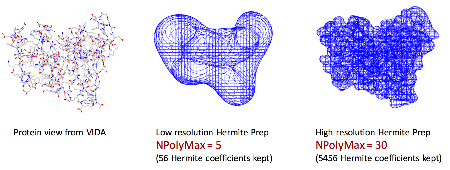
Exact shape versus Hermite Representation
The left figure represents the VIDA view of the exact shape of the protein. The middle figure shows the Hermite representation with NPolyMax = 5. The right figure shows the Hermite representation with NPolyMax = 30. Remarkably, we can encode the main features of the protein shape using Hermite representation with only 56 floating point numbers (middle figure).
The advantages of representing proteins by Hermites include:
smooth representations that capture any level of detail, from the atomistic (many coefficients, as in the picture on the right) to the very coarse (few coefficients, as in the middle picture),
the ability to store these representations in a compact manner,
the ability to transform these representations easily,
very fast overlap calculations between proteins.
Of course, the mathematics of Hermites is more complex than that of a set of atom-centered Gaussians. We have to know how to make, rotate, translate, and scale such representations. Therefore, we are releasing this toolkit with no immediate application or goal - rather, in the spirit of OpenEye, to make potentially useful tools for our customers.
See also
OEHermite class
OEHermiteOptions class
Shape from Hermite expansion examples
Color Features
In addition to shape-alignments Shape TK, optionally, considers chemistry alignment, known as ‘color’. User-specified definitions of chemistry can be included in the superposition and similarity analysis process to facilitate the identification of those compounds that are similar both in shape and chemistry.
Color atoms are described as Gaussians and usually displayed as colored spheres in visualizations. The Gaussian for a color atom is relatively hard with a steep gradient. Figure: Hard vs. Soft Gaussians illustrates hard vs fuzzy Gaussians. Both Gaussians in the figure represent the same volume as the sphere. However, the hard Gaussian, with the steep gradient, reaches a probability of zero (0) within the radius of the sphere. The color features are either matched, if they fall within the sphere radius, or not matched. In the case of the fuzzy Gaussian there are areas outside the volume of the sphere (the area under the curve indicated by the two arrows) where the Gaussian probability is greater than zero. This would allow color features to match even when they align well outside the sphere representing the color atom. That situation would lead to less precise alignments and, for that reason, the ‘hard’ Gaussian is employed.
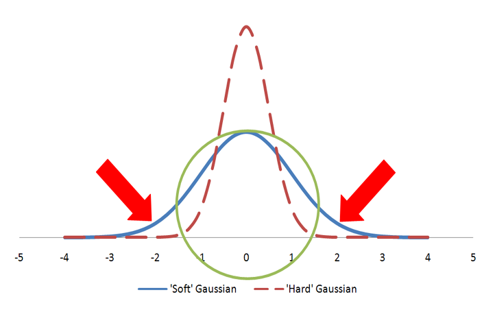
Hard vs. Soft Gaussians
A sphere described by two different Gaussian functions. The ‘hard’ Gaussian (dashed) is the one employed by Shape TK to approximate a color atom sphere.
Shape TK comes pre-loaded with two color force fields, Implicit Mills
Dean (default) and Explicit Mills Dean. These are described in
associated color force field files (*.cff). The desired force field
file can be supplied to the
OEColorForceField.Init method. Further
information on editing color force field files is given in the below
section Color File Format.
The color force field is used to measure chemical similarity between the query and the database molecule and to refine shape-based overlays. The color force field file describes:
Color atom types
- The functional groups to which the color atoms should be applied.
Shape TK uses only the heavy atoms of molecules; hydrogens are ignored.
Whether the interaction between color atoms is attractive or repulsive. Interactions between color atoms of the same type are always attractive. The weight term describes the strength of the interaction relative to the shape gradients and the range term affects the range of the interaction.
The color features described in the Implicit and Explicit Mills Dean color force field files include:
- Donor:
Functional groups that can act as H-bond donors e.g. acid-OH
- Acceptor:
Functional groups that can act as H-bond acceptors e.g. carboxylate
- Anion:
Functional groups with either localized or delocalized negative charge e.g. tetrazole
- Cation:
Functional groups with either localized or delocalized positive charge e.g. guanidinium
- Hydrophobe:
Terminal or non-terminal aromatic or aliphatic groups e.g. phenyl
- Rings:
Rings of defined size e.g. 4-7 atoms
A custom force field file can include other features that you define e.g. positive, negative, carbonyl_linker, metal_binder. For each color atom type a set of SMARTS is used to define the specific functional groups to which the color atom will be applied. The Implicit and Explicit Mills Dean force fields differ in these functional group definitions. For example, the Explicit Mills Dean force field allows a primary amine to be an acceptor as well as a donor whereas it is a donor only in the Implicit Mills Dean force field.
The color force field can also be used for post-shape scoring either alone, e.g. ColorTanimoto and Color Tversky, or in combination with shape scores, e.g. TanimotoCombo and TverskyCombo.
Color File Format
As an alternative to the built-in force fields, the user can define a new color force field using the format described in this section. The following is a simplified example of a color force field specification.
DEFINE hetero [#7,#8,#15,#16]
DEFINE notNearHetero [!#1;!$($hetero);!$(\*[$hetero])]
#
#
TYPE donor
TYPE acceptor
TYPE rings
TYPE positive
TYPE negative
TYPE structural
#
#
PATTERN donor [$hetero;H]
PATTERN acceptor [#8&!$(\*~N~[OD1]),#7&H0;!$([D4]);!$([D3]-\*=,:[$hetero])]
PATTERN rings [R]~1~[R]~[R]~[R]1
PATTERN rings [R]~1~[R]~[R]~[R]~[R]1
PATTERN rings [R]~1~[R]~[R]~[R]~[R]~[R]1
PATTERN rings [R]~1~[R]~[R]~[R]~[R]~[R]~[R]1
PATTERN positive [+,$([N;!$(\*-\*=O)])]
PATTERN negative [-]
PATTERN negative [OD1+0]-[!#7D3]~[OD1+0]
PATTERN negative [OD1+0]-[!#7D4](~[OD1+0])~[OD1+0]
PATTERN structural [$notNearHetero]
#
#
INTERACTION donor donor attractive gaussian weight=1.0 radius=1.0
INTERACTION acceptor acceptor attractive gaussian weight=1.0 radius=1.0
INTERACTION rings rings attractive gaussian weight=1.0 radius=1.0
INTERACTION positive positive attractive gaussian weight=1.0 radius=1.0
INTERACTION negative negative attractive gaussian weight=1.0 radius=1.0
INTERACTION structural structural attractive gaussian weight=1.0 radius=1.0
There are four basic keywords in a cff file: DEFINE, TYPE, PATTERN, and INTERACTION. The TYPE field can be any user-defined term. TYPES can be any user-specified string such as “donor”, “acceptor”, “lipophilic anion” etc. The PATTERN keyword is used to associate SMARTS patterns with these types. There is no restriction on the number of patterns that can be associated with a user defined type. The position in Cartesian space of the PATTERN is taken as the average of the coordinates of the atoms that match the SMARTS pattern. If the desired location of the PATTERN is on a single atom of a larger SMARTS pattern recursive SMARTS (written as ‘[$(SMARTS)]’ can be used to this effect. Only the first atom in a recursive SMARTS pattern ‘matches’ the molecule, and the rest of the SMARTS pattern defines an environment. By writing a SMARTS pattern in recursive notation the location of the PATTERN will be taken as the atomic position of the first matching atom in the pattern. In order to simplify both reading and writing SMARTS, intermediate SMARTS can be associated with words using the DEFINE keyword. Once defined, these words can then be used as atom primitives in subsequent SMARTS patterns with the $ prefix (see “DEFINE hetero” and “PATTERN donor” above).
Interactions between types are associated with the INTERACTION keyword. Two user-defined types must be listed, and whether their interaction is attractive or repulsive. The height and radius can be modified by keywords WEIGHT and RADIUS. At present, the only alternative to a Gaussian decay is invoked by the DISCRETE keyword. A discrete interaction contributes all of WEIGHT if the inter-type distance is less than RADIUS, or zero. Since it is not differentiable it makes no contribution to optimization (i.e. because the gradient of a DISCRETE function is 0 or infinite).
Built-in Color Force Fields
Two color force fields, ImplicitMillsDean and ExplicitMillsDean, are built into the Shape toolkit. Both of these force fields define similar 6 TYPE color force-fields. The types are hydrogen-bond donors, hydrogen-bond acceptors, hydrophobes, anions, cations, and rings. The ImplicitMillsDean force field is recommended.
ImplicitMillsDean includes a simple pKa model that assumes pH=7. It defines cations, anions, donors and acceptors in such a way that they will be assigned the appropriate value independent of the protonation state in the reference or fit molecule. For example, if a molecule contains a carboxylate, ImplicitMillsDean will consider it an anionic center independent of whether it is protonated or deprotonated. This is convenient for searching databases which have not had careful curation of their protonation states. The ExplicitMillsDean file has a similar overall interaction model, however, it does not include a pKa model. It interprets the protonation and charge state of each molecule exactly. Thus, if a sulfate is protonated and neutral, it will not be considered an anion.
The hydrogen-bond models in both ImplicitMillsDean and ExplicitMillsDean are extensions of the original model presented by Mills and Dean [Mills-Dean-1996]. They both have donors and acceptors segregated into strong, moderate and weak categories.
Similarity Measures
Measuring molecular similarity or dissimilarity has two basic components: the representation of molecular characteristics (such as shape and color) and the similarity coefficient that is used to quantify the degree of resemblance between two such representations. Different similarity coefficients quantify different types of structural resemblance.
The table below defines the basic terms that are used in shape-based similarity calculations.
Symbol |
Description |
|---|---|
\(selfA\) |
Self-overlap or self-color score for molecule A |
\(selfB\) |
Self-overlap or self-color score for molecule B |
\(overlapAB\) |
Overlap or color score between molecules A and B |
Tanimoto
Formula:
\(Tanimoto_{A,B} = \frac{overlapAB}{selfA + selfB - overlapAB}\)
The Tanimoto similarity measure is symmetric and always has a value between 0.0 and 1.0 for both shape and color.
Tversky
Formula:
\(Tversky_{A,B} = \frac{overlapAB}{\alpha * selfA + \beta * selfB}\)
The Tversky similarity measure is asymmetric. Setting the parameters \(\alpha = \beta = 0.5\) makes it symmetric and somewhat identical to using the Tanimoto measure.
The factor \(\alpha\) weights the contribution of the first reference molecule. The larger \(\alpha\) becomes, the more weight is put on the self-overlap of the reference molecule.
Unlike Tanimoto similarity, Tversky similarity may not always have a value between 0.0 and 1.0. This is true for both shape and color. Depending on the number of atoms between molecules A and B, it is possible to have \(|overlapAB| > |selfA|\), and that along with certain values of \(\alpha\) can sometimes lead to \(Tversky_{A,B} > 1.0\).
Note
The default settings for RefTversky use \(\alpha = 0.95\) and
\(\beta = 0.05\), and the default settings for FitTversky use
\(\alpha = 0.05\) and \(\beta = 0.95\).
Implementation Details and Usage
Overlap Functions
The overlap functions extend the molecule objective function (OEMolFunc1) interfaces, define in OEFF TK, with overlap interactions, through OEOverlapFuncBase. Similar to the force fields, a shape or a color is also defined as a collection of pairwise interactions. Implementation of overlaps as extension of the molecule objective functions allows for use of the standard optimizers (OEOptimizer1 and/or OEOptimizer2) for minimization of overlaps and corresponding quantities. Implementation of overlaps as extension of the molecule objective functions also allows for combining the overlap functions with other molecule objective functions, such as the force fields, for system optimization. An overlap function in Shape TK can consist of just shape or color, or a combination of both.
The overlap functions are the simplest objects in Shape TK, and can is used to calculate simple, static, overlap between two objects (molecules, grids or shape queries). Note that static means that the two input species (ref and fit) are not moved at all. These objects simply calculate the static overlap, gradients and other corresponding quantities, given the input positions.
Overlap Methods
Three different algorithms are implemented to calculate the overlap and the corresponding gradients, between two gaussians, that provides a balance between accuracy and speed.
The Exact option considers all pairs of atoms in the system, and the Gaussian overlaps are calculated exactly.
The Analytic option provides multiple options to approximate the calculations. The first option corresponds to using a pre-calculated table for estimating the exponentials vs. doing exact calculation of the exponentials. The second option allows to use a proximity grid to only consider those atom pairs that are within a certain threshold distance (by default 3.0 Å). The average error introduced by either of these approximations is in the order of one part in a thousand. The speed gain from the proximity grid increases with size of the molecules, as well as with the number of overlap calculations performed. The later is related to the increased setup time for the proximity grid for the reference molecule. If both the tabulated exponentials and the proximity grid is turned off, the Analytic option simply folds back to the Exact option.
The final option, Grid, uses a grid representation of the volume of the target molecule. It requires significant set-up time relative to the cost of a single overlap calculation (~0.01s compared to ~0.0001s) but is significantly faster than other methods for the evaluation of each overlap once set. Grid suffers a few caveats and drawbacks. First is that, currently, for shape overlap calculation, all atoms are treated as if they have the same radius (that assigned to carbon). The second is that the approximation is slightly worse, typically a few parts in a thousand, at typical grid resolutions.
Both Analytic and Grid improve performance when the fit molecule is large (>20 atoms) because, if there are n atoms in the fit and m in the reference, the work per atom in the fit is proportional to a constant not n.
Besides the Gaussian based calculations, a fourth option, Hermite is available for shape overlap calculation, based on Hermite representation of shape as described above earlier.
Radii approximations
Since we are considering molecular volume overlap as a measure of shape, the
radii used for each atom is important. There are essentially two
settings. A radii approximation of OEOverlapRadii_All
means each atom will be treated with the radius as passed
in. Alternatively, one can treat all heavy atoms as similar and apply
the OEOverlapRadii_Carbon radius approximation. With
this, all heavy atoms will be assigned the same radius, regardless of
the value attached to each atom. As noted above, if the
Grid method is used for overlap calculation, only the
OEOverlapRadii_Carbon radius approximation can be used.
Overlap Optimization and Overlay
Two high level objects, OEROCS and OEOverlay are provided for optimizing a OEOverlapFuncBase, to maximize shape (and color) overlap between two objects and obtain the best overlay. Both the OEROCS and OEOverlay optimizes the overlap between the reference and fit object, but provides different level of usability.
Starting positions for optimization
The starting points are important for any optimization. Various options to start an overlap optimization is provided through the OEStarts interface. The reference structure is always aligned by its principal moments of inertia, and the initial alignments of fit structure is determined by the specified options.
In the Inertial start, in general, the fit object is aligned in 4 positions with the primary and secondary moments of inertia in both directions. In order to deal with structures with symmetrical moments of inertia, additional starting points are generated. For a reference or fit where the 2 major moments of inertia are equal (to a user-defined percent, nominally 15%), 4 extra starting positions are generated. In the rare case of a molecule with all 3 moments of inertia essentially equal, 20 random starting translations and rotations are chosen as starting positions. For virtual screening uses, where the reference and fit molecule are similar in size, the inertial starts provide an excellent choice for starting positions that balances quality results with speed.
There are times when there is a large difference in size and a more elaborate search is needed. For these, there are a couple of built-in searches as well a user-defined search. To increase searching, instead of doing the inertial frame rotations with to 2 molecule centers-of-mass (COM) aligned, we can do a set of inertial rotations at many more locations.
The AtAtom starts will translate the COM of the fit molecule to the specified atom center (usually the heavy atoms) locations of the reference molecule. At each of these translations, it will perform the 4 basic inertial transforms. Note that this means that instead of 4 (or 8) starting positions, there will be 4 x number of reference molecule heavy atoms (or what other atom centers specified) starts, resulting in 20-30 more starting positions compared to the Inertial starts. Obviously this will slow the overall calculation so this is not recommended for high-volume virtual screening, but is very useful for low-volume fragment searching. A slightly less aggressive set of starting positions can be to use the color atom centers instead of the heavy atoms of the reference molecule. For an average reference molecule with ~10 color atoms, this will be faster than using all heavy atom positions, but not as elaborate of a search.
The Subrocs starts automatically performs AtAtom starts on each heavy atom of the larger molecule, regardless of which molecule is set as the reference.
With the Cartesian starts, the user can specify the points at which to translate the fit molecule before doing the 4 basic inertial transforms. This provides more flexibility in terms of how to starts to do for any optimization.
The Random starts, will generate N random starting positions where N is user-defined, as well as the maximum translation allowed between random starts. The fit molecule will be translated to these random starting positions, and the basic inertial transforms will be applied.
The AsIs starts gives the option to the user to start the optimization from a single, pre-aligned position.
And finally, the Quat starts takes the user specified quaternions as the transformations to be applied to the fit molecule before performing optimizations.
Thus, for any given optimization, there are multiple results returned, usually only one of which is useful.
Preparing Molecules
Tools for preparing molecules are provided separately so users can prepare their molecules once and reuse those molecules for many calculations. However, the high level OEROCS object for overlay optimization also provides a convenient option to automatically prepare molecules, if desired.
There are essentially three components to preparing molecules.
The first is to choose either to have hydrogens explicitly or not, and add or remove the hydrogens in the molecules. Shape is a heavy atom property and most OpenEye uses (as well as the default option in OEOverlapPrep) is to ignore the hydrogens.
The second is to assign Bondi radii on the atoms, if desired. This is required if
a radii approximation of OEOverlapRadii_All is to be used for
shape overlap calculations.
The third is to choose to have color atoms or not. Even if color is used for the calculations,
it is possible to have user defined color atoms on the molecules and direct OEOverlapPrep
to not make modifications to them (see OEOverlapPrep.SetAssignColor).