Tutorials
The following tutorials are intended as quick start guides to Orion.
An Orion Docking Workflow
This tutorial shows use of a sequence of floes to perform a project. It also shows how to use an assortment of user interface features, such as examination of binding sites.
DNA gyrase (GyrB) and topoisomerase IV (Topo IV) are clinically validated targets for the treatment of resistant bacterial infections. In a study carried out at a big Pharma, pyrrolamides were shown to exhibit antibacterial activity by competing with adenosine triphosphate (ATP) in DNA gyrase and Topo IV.
In this simulation, your role as the only modeler on the pyrrolamides optimization project is to guide the medicinal chemists in their design decisions; they want suggestions on what to synthesize next. Your ultimate goal is to help them synthesize the depicted compound.
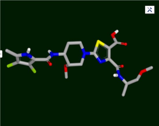
Figure 1: Target Compound
You will explore docking in this retrospective study. In the drug discovery process, structure-based methods such as docking—the lock-and-key concept where the protein is the lock and the ligand is the key—use the structure of a target protein to discover hits and optimize leads. In hit discovery or virtual screening, no molecules are known that are active against the target protein. Docking is used to identify possible active molecules in a large molecule database, by examining their shapes and chemical complementarity to the active site.
Datasets
Initial ligands: pyrrolamides_3D.sdf – download the dataset below.
Receptor: 3TTZ_A_receptor – download the receptor below.
Conformer database – generate from pyrrolamides_3D dataset (see below).
Download dataset of initial ligands
Download receptor
After completing this task, you will be able to:
Upload datasets into Orion
Run an Omega floe
Retrieve a receptor from a database
Identify the binding pocket
Perceive protein-ligand interactions
Run a docking floe
Analyze docking results in the
AnalyzepagePerform a substructure search
Add property data to a spreadsheet
Sort the data in a spreadsheet
Export data
Navigate to the Orion Home page and create a project called “Docking Demo.”
Figure 2. By Default, Orion Switches to the New Project Automatically
Navigate to the
Data(Project Data) page and upload the ligand file pyrrolamides_3D.sdf.
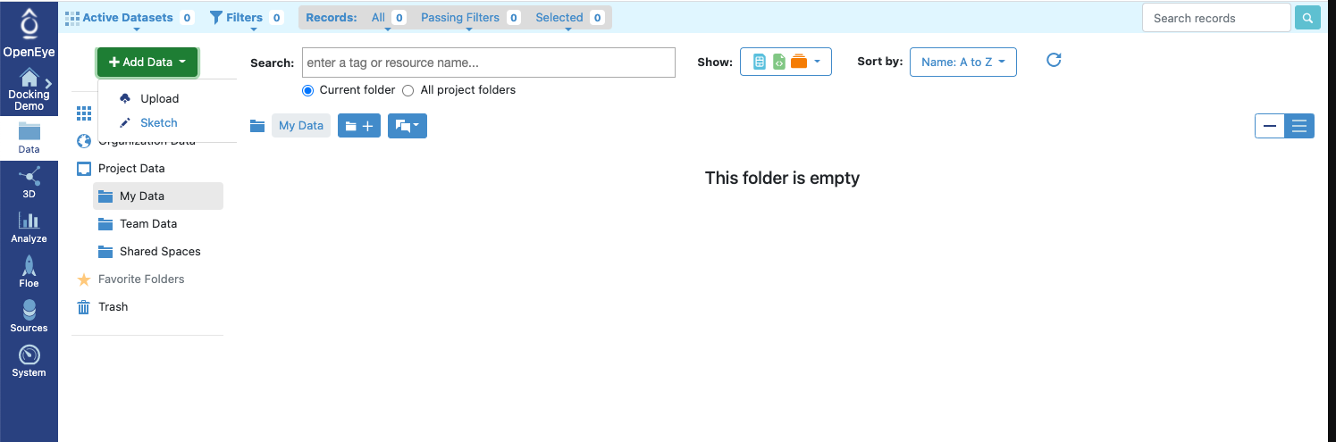
Figure 3: Adding Data
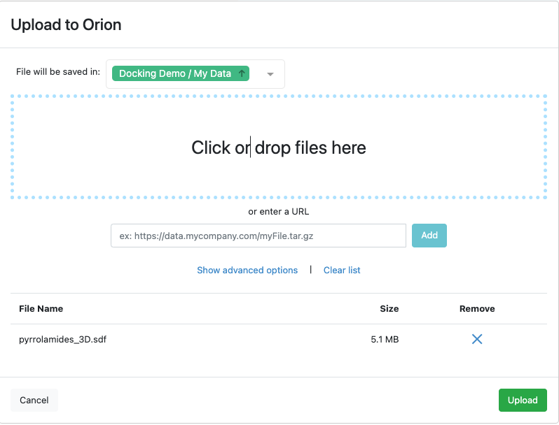
Figure 4: Ready to Upload a File of Data
A dialog pops up showing that the upload is in progress, then a conversion floe, File to Dataset Import, runs quickly, producing a dataset from the uploaded file.
You can see the recent notifications by clicking the Notifications icon ( ).
).
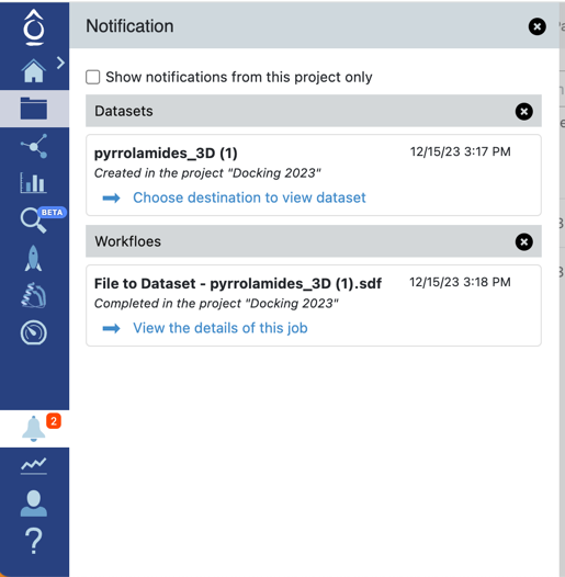
Figure 5: Notification List
The end result is shown here.
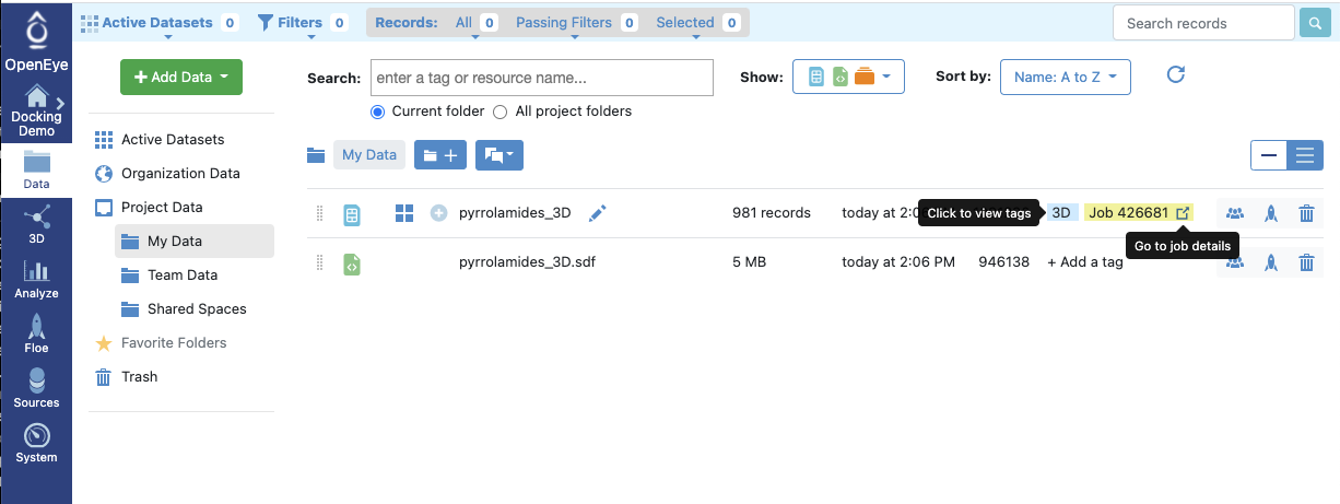
Figure 6: Requesting Job Details
The icon next to the job details on the upper right ( ) shows the job that produced the dataset. A job is
an instance of a workflow, or floe, in this case the format conversion floe File to Dataset Import.
) shows the job that produced the dataset. A job is
an instance of a workflow, or floe, in this case the format conversion floe File to Dataset Import.
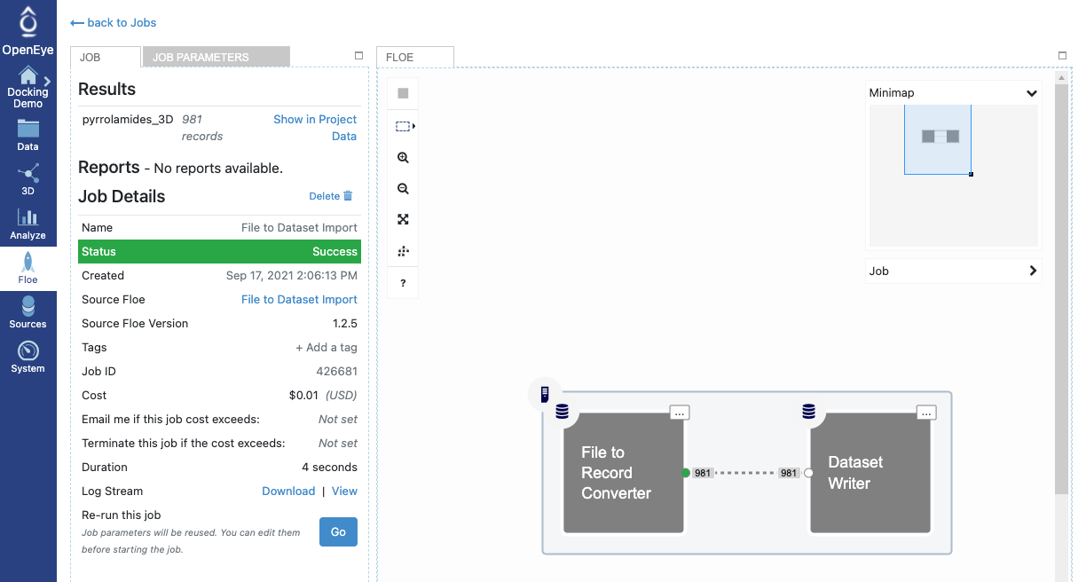
Figure 7: A Successfully Completed Job
Here, a File to Record Converter cube uploaded and converted the ligand file and then it fed its output to the Dataset Writer cube.
Switch to the
Floe(Workfloe) page, select theOMEGA - 3D Conformer Ensemble GenerationFloe and generate ligand conformers.
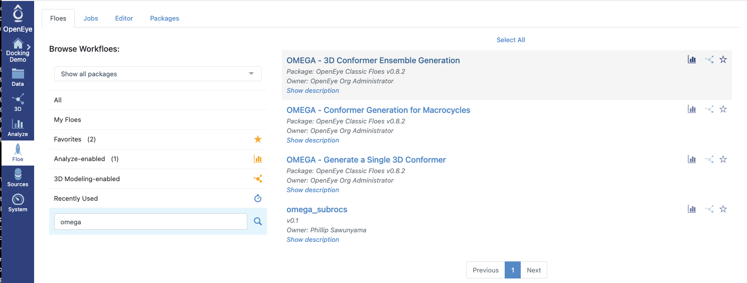
Figure 8: Listing Floes That Use Omega
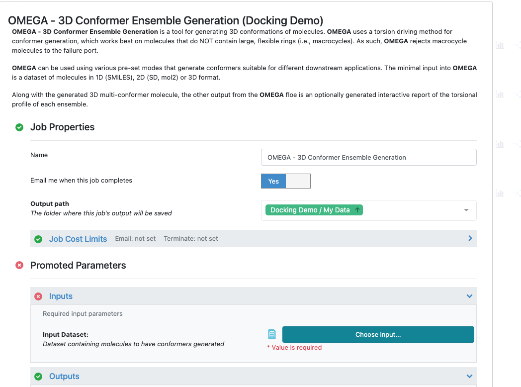
Figure 9: Launching a Specific Omega Floe
Click on the Choose input... button, and the screen will navigate to your My Data folder in the project data.
Select the pyrrolamides_3D file as input to the OMEGA - 3D Conformer Ensemble Generation floe.
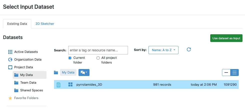
Figure 10: Selecting an Input Dataset
Click on the name pyrrolamides_3D to select that file, and then click the  icon to provide it as input
to the floe. You can leave the other parameters with their default values and click the icon.
icon to provide it as input
to the floe. You can leave the other parameters with their default values and click the icon.
The floe runs for only a few minutes, after which there is a new dataset—the set of conformers—in your data folder.
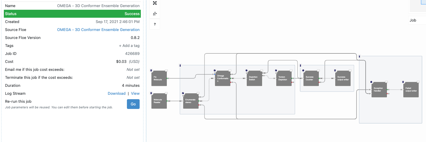
Figure 11: Job Details for an Omega Floe
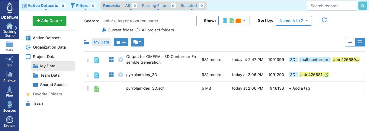
Figure 12: Output of an Omega Floe
5. To prepare the receptor, click on the  icon, then select the file
 3TTZ_A__receptor.oeb at the location to
which you downloaded it previously. After another run of the File to Dataset Import floe, the receptor data are
present in the project’s My Data folder.
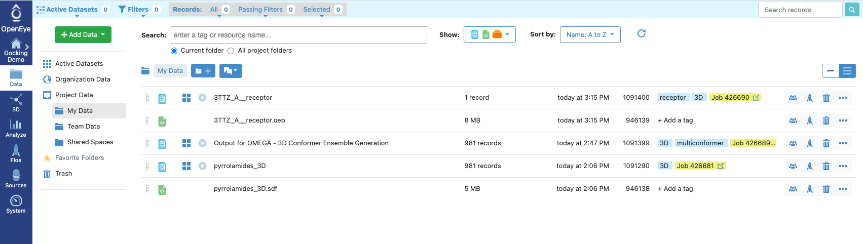
Figure 13: Receptor Provided
We have provided the receptor file as a download in this tutorial, but more typically you might click on
the Macro Molecules
page and get a receptor from a database such as MMDS.
Generate a binding site.
Verify that the 3TTZ_A_receptor is now available in the
Active Datasetslist on theProject Datapage.Click on the
 icon next to the 3TTZ_A_receptor name. This adds the receptor
to the active dataset(s).
icon next to the 3TTZ_A_receptor name. This adds the receptor
to the active dataset(s).
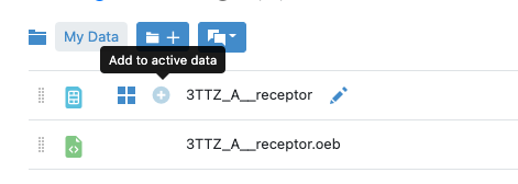
Figure 14: Adding the Receptor to the Active Datasets List
Go to the
3D Modelingpage and examine the binding site.
To make the receptor and ligand visible, click on the Show/Hide icons for the receptor and the ligand 07N(A), respectively.
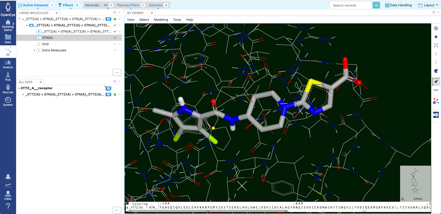
Figure 15: Showing the Receptor and Ligand
Generate the Binding Site view:
With receptor selected,
With ligand 07N(A) selected,
Click the Generate Binding Site icon (
 )
)
You can control elements of the displayed binding site wih the
Binding Site Optionsdrop-down. (Click on the bar under the icon.) For example,
you can uncheck Show Labels?and then regenerate the binding site.
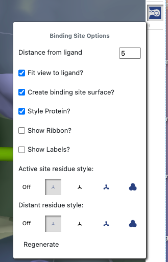
Figure 16: Binding Site Options
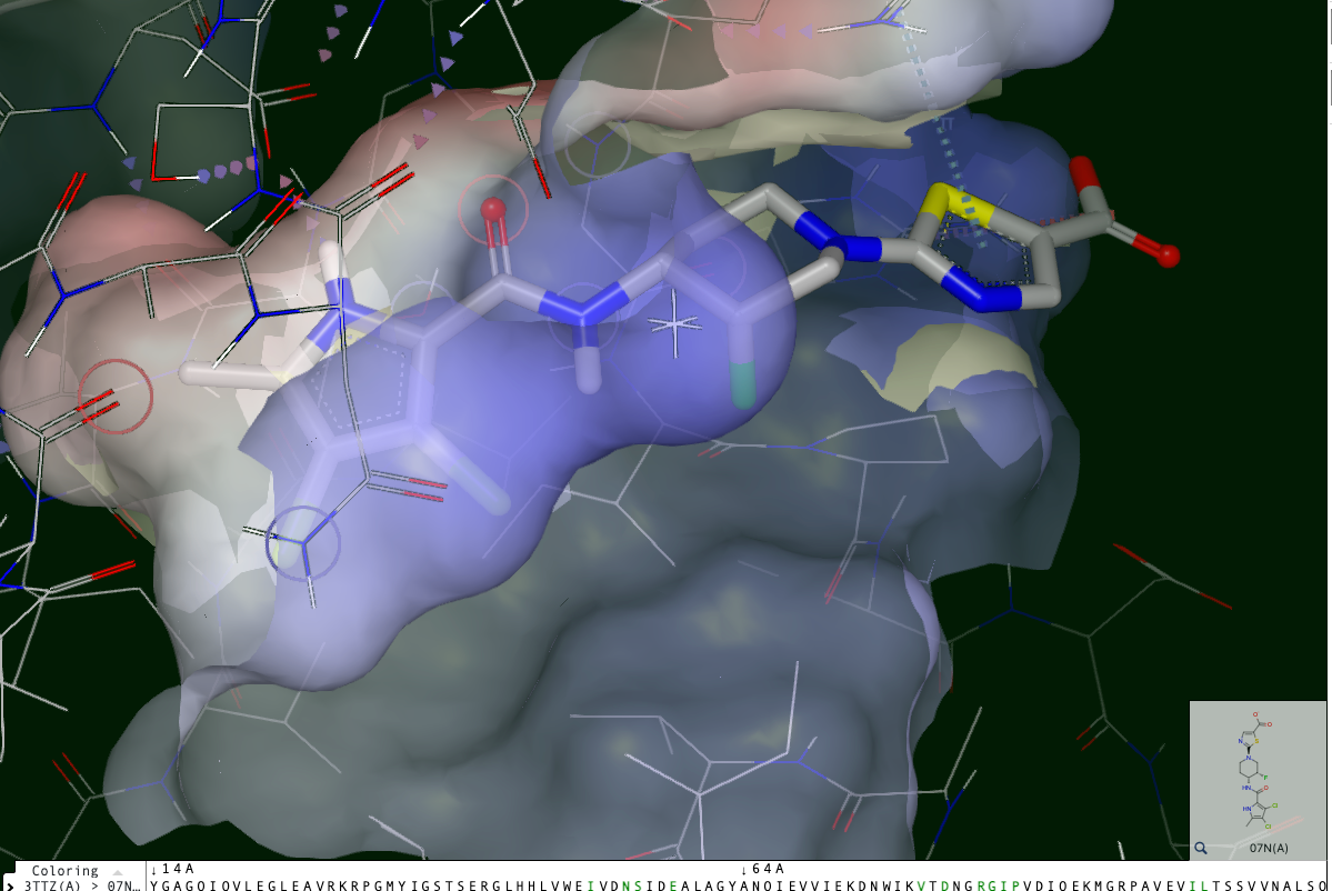
Figure 17: A View of the Binding Site
Examine the protein-ligand interactions. The auto-interactions icon (
 )
has a drop-down with additional display options.
)
has a drop-down with additional display options.
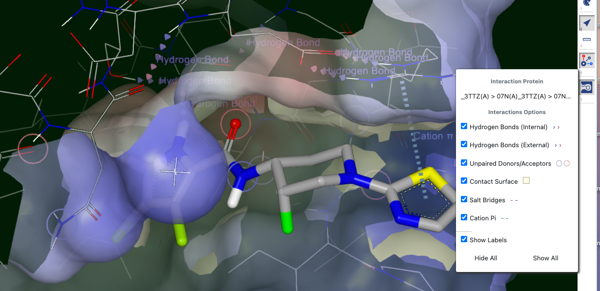
Figure 18: Interactions and Options
10. Launch the Docking Floe:
Switch to the Floe page and
select the OEDocking - Dock into an Active Site for Virtual Screening Floe.
You may need to do a search for “OEDocking” to bring up this floe on the selection list.
Enter the docking inputs, and click
Start Job.
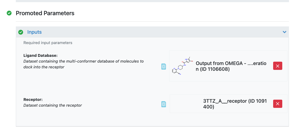
Figure 19: Inputs to the Docking Floe
The job typically completes in about 10 minutes.
Add docked poses to active datasets:
Once the docking job is complete, click
Project Data.Add 3TTZ_A-07N_A_373_receptor to Active datasets.
Add pyrrolamides_3D_docked_into_3TTZ to Active datasets.
Analyze the results.
Go to the
Analyzepage. Make a scatter plot with Chemgauss on the Y axis and IC50 on the X axis.
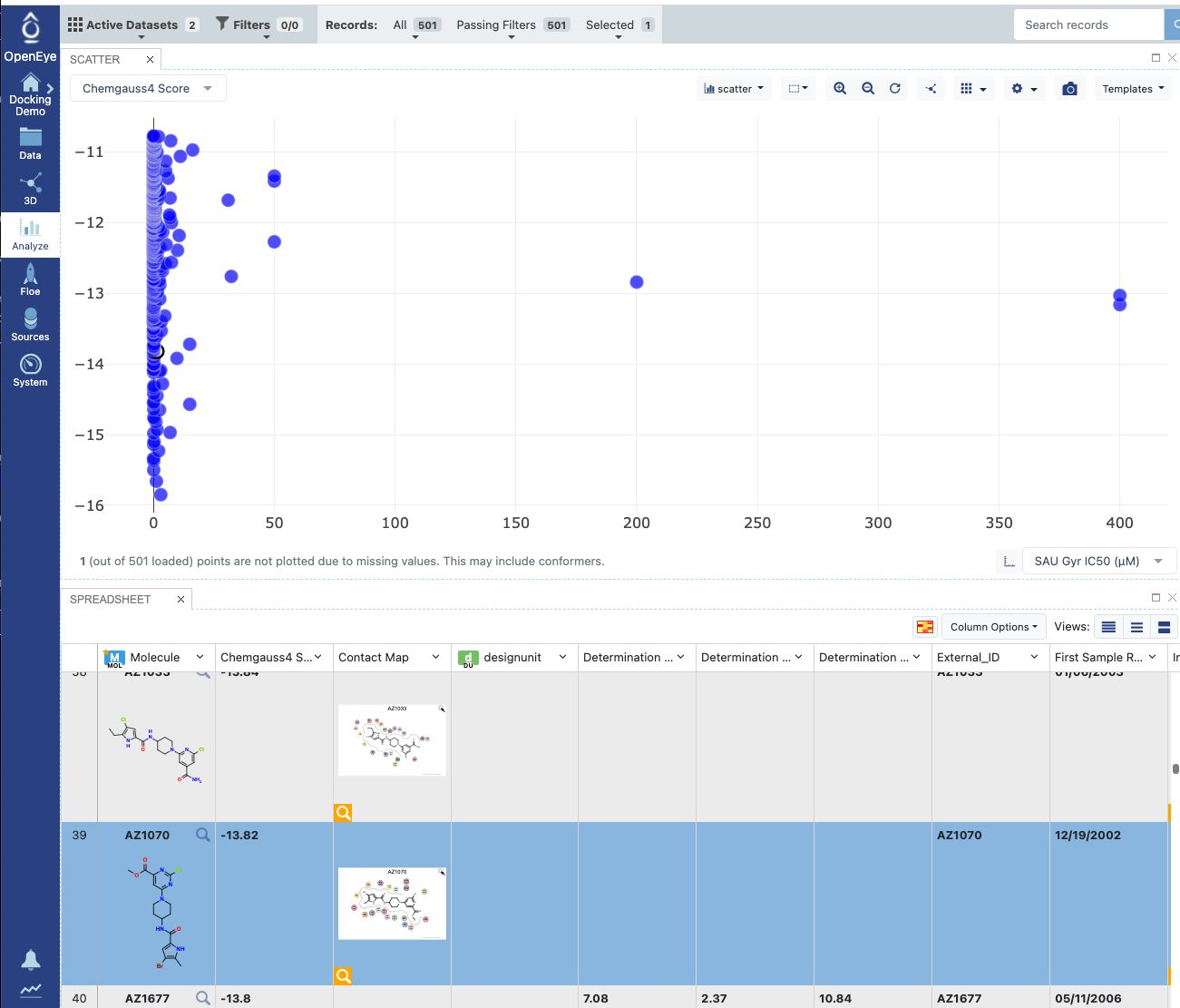
Figure 20: Analyzing in a Scatter Plot
To show a depiction of a molecule, you can scroll to it in the list
in the bottom part of the Analyze page and click on the  icon.
icon.
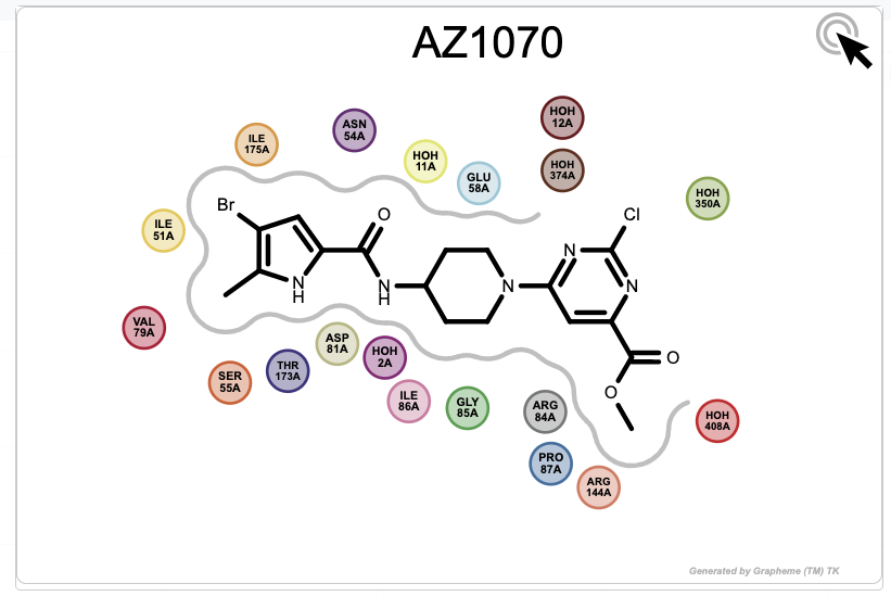
Figure 21: Magnified Depiction of a Molecule
Examine Docked Poses.
Go to the
3Dpage.
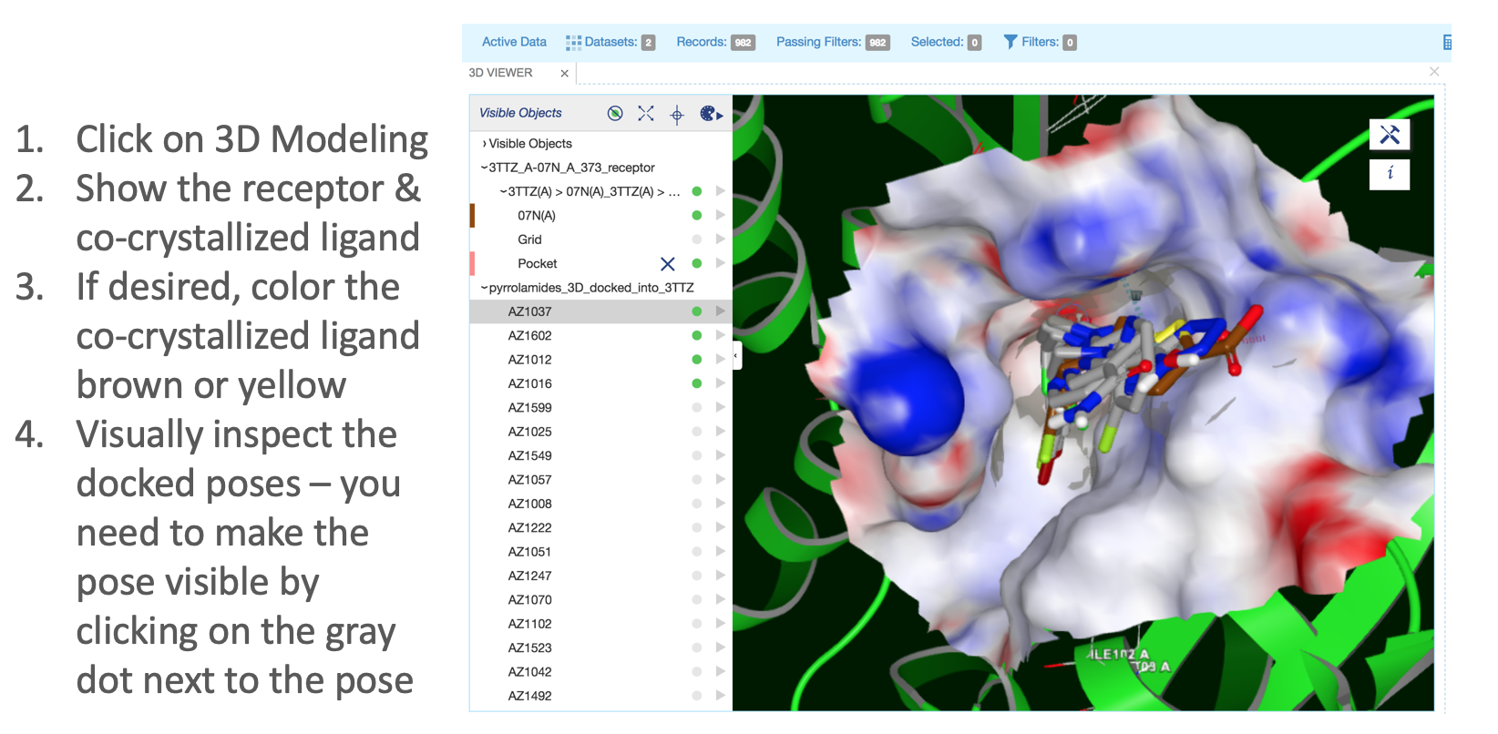
Figure 22: Docked Poses
Background Information about Docking
Would you like to know more?
For more information about the Classic Docking Floe, see OEDocking–Dock into an Active Site for Virtual Screening.
For more information about the Classic Omega Floe, see the reference documentation about the Omega Floe used in this tutorial.
If you are doing more advanced work in Python, you may also be interested in the theory of docking, as presented here.