3D & Analyze Page
Note
The 3D & Analyze page offers a streamlined approach to data analysis by combining the tools from the previous 3D Modeling and Analyze pages into one page. Users can now visualize and analyze data without moving between different pages. Keyboard shortcuts allow you to switch easily between preset layouts that previously were on different pages.
The 3D & Analyze page provides several ways to examine and interact with data.
The 3D Viewer allows the user to interact with and edit molecular structures, examine docking results, perceive protein-ligand interactions, and edit ligands in the context of the active site. Data trees accompanying the 3D Viewer show molecules, proteins, and related information such as constraints.
The 3D & Analyze page also includes an interactive molecular spreadsheet. It allows typical actions such as column sorting, pinning, and choice of selected rows.
Graphing capabilities offer several plot types, including scatter, boxplot, and histogram, as well as robust multi-linear regression. The 3D Viewer, spreadsheet, and plots are connected such that a molecule selected in one is also active in the other two.
Numerous cheminformatics functions are available, such as substructure search, R-group decomposition, and property calculation. Floes to calculate new properties for plotting and regression can be called directly from this page.
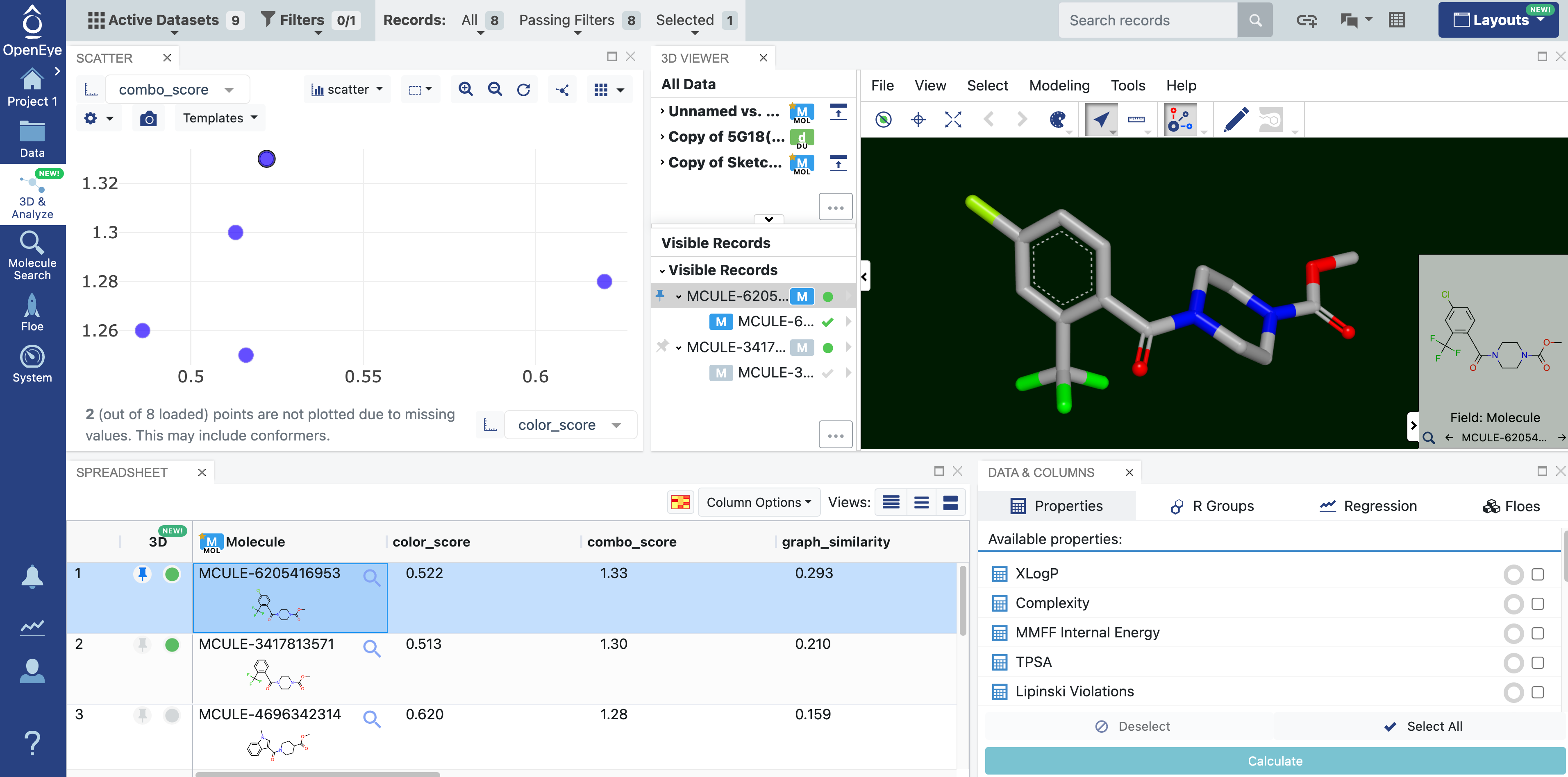
Figure 1. The 3D & Analyze page showing the 3D Analyze view plus the Data & Columns panel. Different views can be toggled using keyboard shortcuts or via the Layouts drop-down. In this case, the Data & Columns panel was added to the preset 3D Analyze view by clicking on “data & columns” in the Layouts drop-down.
Table 1. Important Features of the 3D & Analyze page.
Name |
Description |
|---|---|
3D Viewer |
Displays 3D structures of small molecules, macromolecules, design units, and other 3D objects. |
Spreadsheet |
Displays imported data, molecular structures, and images. Users can include a variety of column options
and calculated properties, such as PSA and XLogP.
|
Plot |
Allows users to create plots. The plot type (scatter, boxplot, heatmap, histogram, or violin) can be
selected from the Plot drop-down menu.
|
Data & Columns Panel |
Allows users to compute molecular properties, perform R-group decomposition, and predict properties using
a regression model.
|
Active Data Bar |
Offers a variety of tools, including the rapid switching between active datasets, filtering, data handling,
and managing page layouts.
|
Layouts Drop-Down |
Allows users to customize the panels on the page, including preset views (3D Analyze, Analyze, and 3D
Modeling). Other layouts or features can be added via click or drag-and-drop.
|
3D Viewer Toolbar |
Allows users to fit objects in the Viewer, style molecules and proteins, change mouse modes, perform
measurements, edit small molecules, select protein interactions, and generate and
manipulate a binding site of a selected receptor.
|
3D Viewer Data Trees |
Allow users to view and utilize molecule information in the 3D Viewer. These lists include All Data,
Focused Data, Pinned Data, Large Molecules, Visible Records, and Visible Objects.
|
Files can be uploaded directly to the 3D & Analyze page using a drag-drop feature. A checkbox also allows a dataset to be added to Active Data when file upload is complete. This option is defaulted to Off. While the Add to Active Data feature is off by default, the UI will retain the selection and the checkbox will remain checked if it was used for the previous upload. Be sure to review the selection before uploading a file.
Data Panel Shortcuts
Four primary data panels are available on the 3D & Analyze page: 3D Viewer, Spreadsheet, Plot, and Data & Columns. Three preset views are offered under the Layouts drop-down: 3D Analyze, Analyze, and 3D Modeling. Clicking on the Layouts button brings up all possible panel options and selecting a panel will add it to the screen. Clicking the X in the corner of a panel removes that panel from the current page view.
Note
Keyboard shortcuts can be used to easily switch between default views.
Table 2. Keyboard shortcuts for toggling 3D and Analyze views.
Mac Keyboard Shortcuts |
Windows Keyboard Shortcuts |
Layout View |
Panels |
|---|---|---|---|
Option + 1 |
Alt + 1 |
3D Analyze |
3D Viewer, Spreadsheet, Plot |
Option + 2 |
Alt + 2 |
Analyze |
Spreadsheet, Plot, Data & Columns |
Option + 3 |
Alt + 3 |
3D Modeling |
3D Viewer |
With a variety of movable panels that can be selected, hidden, or resized as needed, the 3D & Analyze page offers maximal flexibility for examining data.
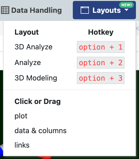
Figure 2. The Layouts drop-down showing Mac keyboard shortcuts for 3D & Analyze page views. See Table 2 above for Windows shortcuts.
Active Data Bar
The Active Data Bar contains several useful drop-down menus and features. It allows the selection of active datasets, filtering of records, data handling, layout options, and more. The Data page also contains an Active Data Bar.

Figure 3. The Active Data Bar.
Active Datasets
The Active Datasets drop-down allows rapid selection of and toggling between multiple datasets. If no datasets are activated, then no data will be populated. To browse datasets, click the Active Datasets drop-down.
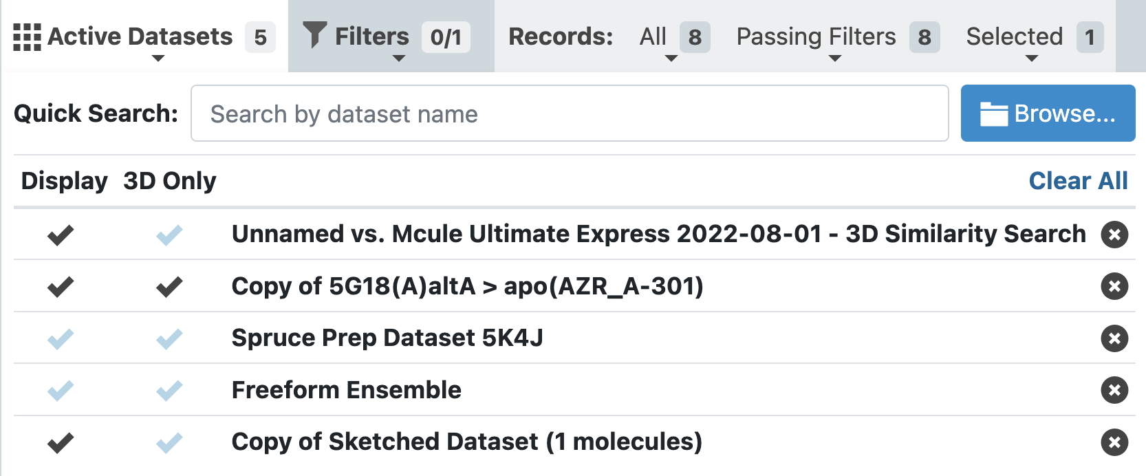
Figure 4. The Active Datasets drop-down. Datasets that are checked under “Display” will appear in the Spreadsheet, Plot, and 3D Viewer. Those checked under “3D Only” will appear only in the 3D Viewer. Datasets with grey checkmarks are active, but not displayed in the 3D & Analyze page.
If a dataset is listed, click the corresponding checkmark under “Display” to display it.
If the dataset is not listed, type the name into the Quick Search bar, or click the “Browse” button to select a dataset from the Data page.
For each dataset in the Active Datasets drop-down, you can check “Display” to show all data in that dataset or uncheck to hide a dataset without deactivating it.
The “3D Only” option allows for data to be hidden from the Spreadsheet and the Plot while still appearing on the 3D Viewer and 3D Viewer data lists. This may be useful when working with docking results, in order to hide extra columns that are part of a DU but not part of each molecule in a docking hit list. A dataset that is selected as “3D Only” will appear in the Focused Data list. It also excludes that dataset from any filtering.
Individual datasets can be cleared by clicking the X, and all datasets can be cleared by selecting the “Clear All” button.
Please notes that datasets with over 100,000 records are not recommended for use in the 3D & Analyze page.
Filters
Using the Filters drop-down, two types of filters may be applied to the active and displayed datasets. The number of active filters is shown on the Active Data Bar.
Note
For all filter queries, the “Enabled” box must be checked to filter all molecules that are active and displayed. The “Invert” checkbox filters all active and displayed molecules that do not have that substructure.
Enabled filters from previous queries on any active datasets will appear in the drop-down and will be applied to all active and displayed datasets.
To apply a filter, click on the Filters drop-down, then the ‘Choose a Filter’ box. Two categories will be available, substructure and column. Any previous or current substructure filters and all column options will be visible. Enabled filters for each category can be collapsed.
The first type of filter is a substructure filter. For a new query, click on the New Query button to open the Sketcher; a query name is required to search for that substructure.
The second type of filter is based on data in the columns of the related spreadsheet. These filters (columns) vary with the dataset and may include data such as molecular weight, heavy atom count, and Tanimoto combo score. Some qualities, such as molecule or PDB, offer an option to enter a query name; a name must be provided to apply the filter. For others, such as chiral centers or Tanimoto combo score, a value or range of values must be provided. Certain column filters give the option to view the information in a list or visualize it in a histogram.
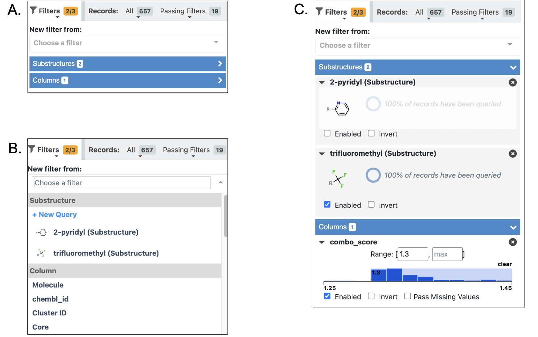
Figure 5. The Filters drop-down. A. Drop-down with filter options collapsed. B. Available filter options, including existing substructure filters, an option for a new substructure filter query, and column filters. C. Expanded filter options showing the details and enabled status of existing filters. Along the top, the Active Data Bar shows the active versus total filters (2/3), the number of records filtered (657), and the number passing filters (19).
Categorical string fields can be filtered using a “free text” setting. This allows creation of filters that can match multiple distinct categorical values that contain a provided string.
Records
The Records drop-down includes three parts: All, Passing Filters, and Selected. The number of records that match each part is displayed at the top. The All drop-down allows for working with all of the active datasets, whether they are displayed or not; these records can be sent to a floe, saved to a new dataset, or appended to an existing dataset. The Passing Filters drop-down allows for tagging, sending to a floe, saving to a new dataset, or appending to an existing dataset only the records that pass a chosen filter. The Selected drop-down is similar to the Passing Filters drop-down, but is only for records that are highlighted and selected.
Snapshot Link
The Snapshot Link option allows you to create a link to the current state of the 3D & Analyze page, either to share that page with other project members or to return to the same state after switching to a different project or task.
Discussion Boards
You often need to share data and discuss the results with team members. Discussion boards are accessed by the “chat” icon on the Active Data Bar. This drop-down allows you to create and access your discussion boards. They are organized by project name and are also available on the Data page. Discussions are preserved so you can revisit them. The discussion board autosaves users’ edits.
You can share links and images along with text comments. A snapshot from the 3D & Analyze page can be included on a discussion board. Snapshot links can be added in two ways. First, you can select text while writing a discussion comment and click the ‘Snapshot link’ tooltip. This link style will open in the same tab as your current session. Alternatively, you can click the Snapshot icon in the Active Data Bar and paste it into the comment: that link will open in a new tab.
For more information, see the training video for using discussion boards.
Data Handling
The Data Handling feature enables the user to manipulate data in the Spreadsheet. The visibility of columns across all displayed datasets can be selected here. Data can appear in all settings, or it can be selected separately for visibility in 3D, the spreadsheet, or the plot. It also provides style options for the treatment of imprecise data (e.g., ranges, inequalities, and multiple values). Data Handling shows data completeness for each column, as well as the type of the column (string, int, float, etc.).
If multiple molecule fields are present, you can toggle between the options to choose which molecule should be the primary molecule.
After making changes in the Data Handling modal, click the “Apply” button.
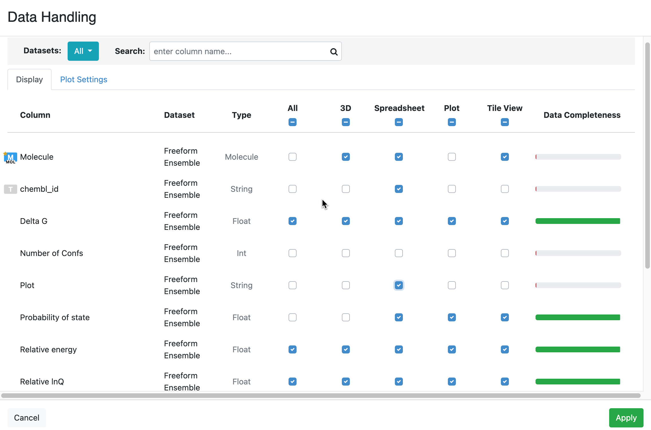
Figure 6. The Data Handling window. Visibility of features in 3D, spreadsheet, plot, and tile view can be selected or deselected either singly or for all columns at once. This image shows
This feature can be accessed from either the Active Data Bar or the ‘Column Options’ drop-down in the Spreadsheet. For more information about using the Data Handling tool, see the Spreadsheet section.
Layouts
The Layouts drop-down allows users to choose the panels on the page, including both standard layouts and additional options that can be clicked or dragged onto the page.
The primary data panels on the 3D & Analyze page are the 3D Viewer, Spreadsheet, Plot, and Data & Columns. Table 2 defines preset views that are available using these panels, along with their keyboard shortcuts. Clicking on the Layouts button brings up the preset views, panels that aren’t visible in the current page view, and two secondary options, Job History and Links, which can be added to any layout. Selecting a panel adds it to the screen; to control the location of the panel, drag it in rather than clicking on it. All panels can be dragged to reposition as desired. Clicking the X in the corner of a panel removes that panel from the current page view.
Custom layouts can be created and saved. This feature is useful if you often work with specific panels in a particular arrangement that is not available in a preset layout. The custom layout will appear in the Layouts drop-down menu along with its own hotkey (e.g., “spreadsheet only” in Figure 7). Preset views can be restored by clicking the revert button in the Layouts drop-down.
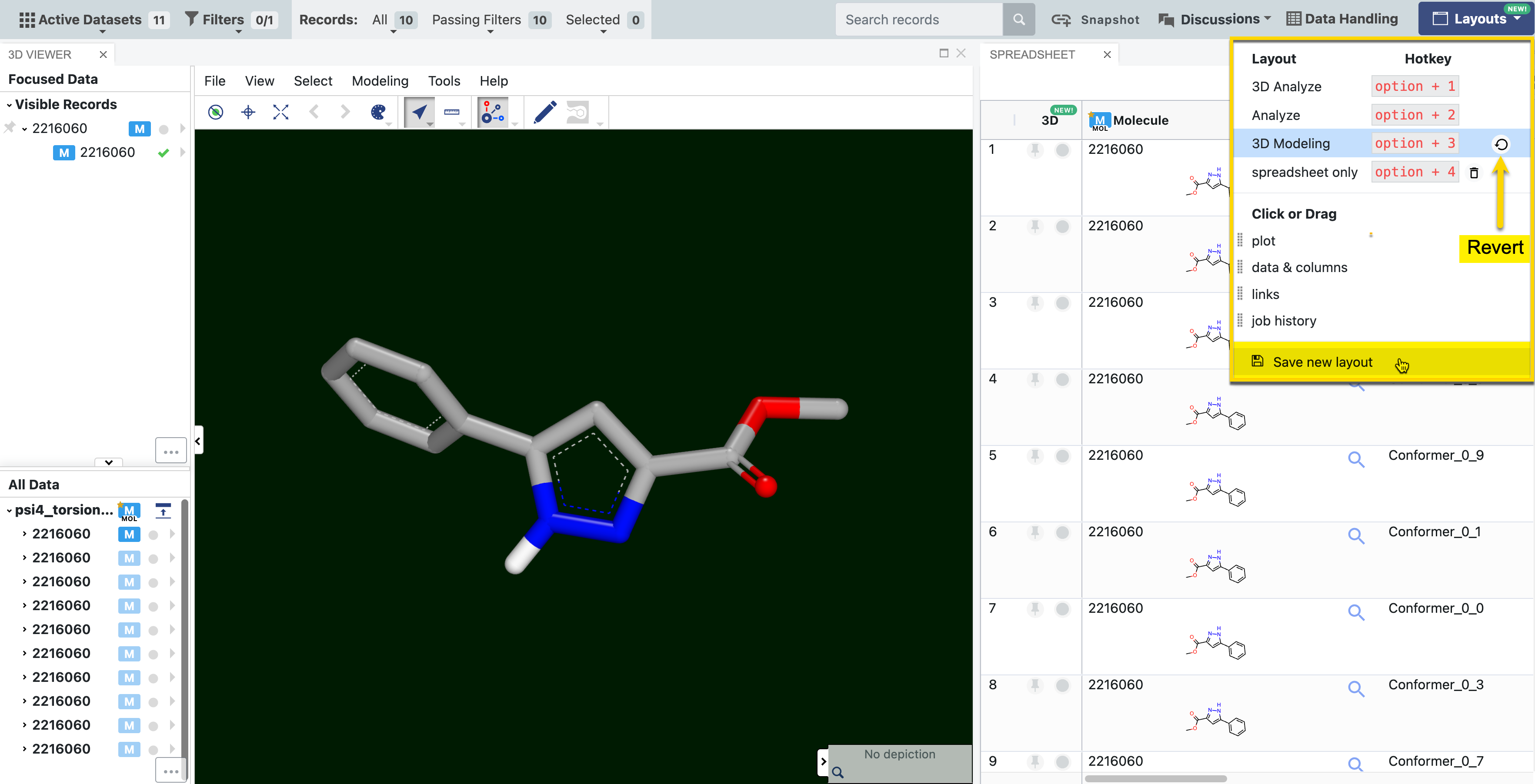
Figure 7. Saving a custom layout. The “Save new layout” button enables the user to save a unique layout, such as the side-by-side view of the 3D Viewer and Spreadsheet panels shown here. The preset 3D Modeling view can be restored by clicking the revert button.
Keyboard shortcuts allow you to easily toggle between the preset layouts. Custom layouts can also be accessed using keyboard shortcuts. For Windows machines, use Alt rather than Option.
Option + 1: 3D Analyze (Default view)
Option + 2: Analyze
Option + 3: 3D Modeling
Option + 4 (and up): Custom Layouts
Spreadsheet
The Spreadsheet allows typical actions like column sorting, pinning, reordering or deleting, and choice of selected rows. Columns can be moved, deleted or hidden. Spreadsheet cells can be copied to the clipboard, sent to other tasks in Orion, rated, and tagged. Pop-out views of structures are also available by clicking on the magnifying glass icon. Records in a dataset can be deleted directly from the Spreadsheet or from the 3D Viewer data trees. To delete from the Spreadsheet, right click in the record and select Delete. From the 3D Viewer data trees, expand the caret next to the record name to reveal the side menu. Click the Data Operations folder icon and choose “Delete this record.” Please note that deleting a record cannot be undone.
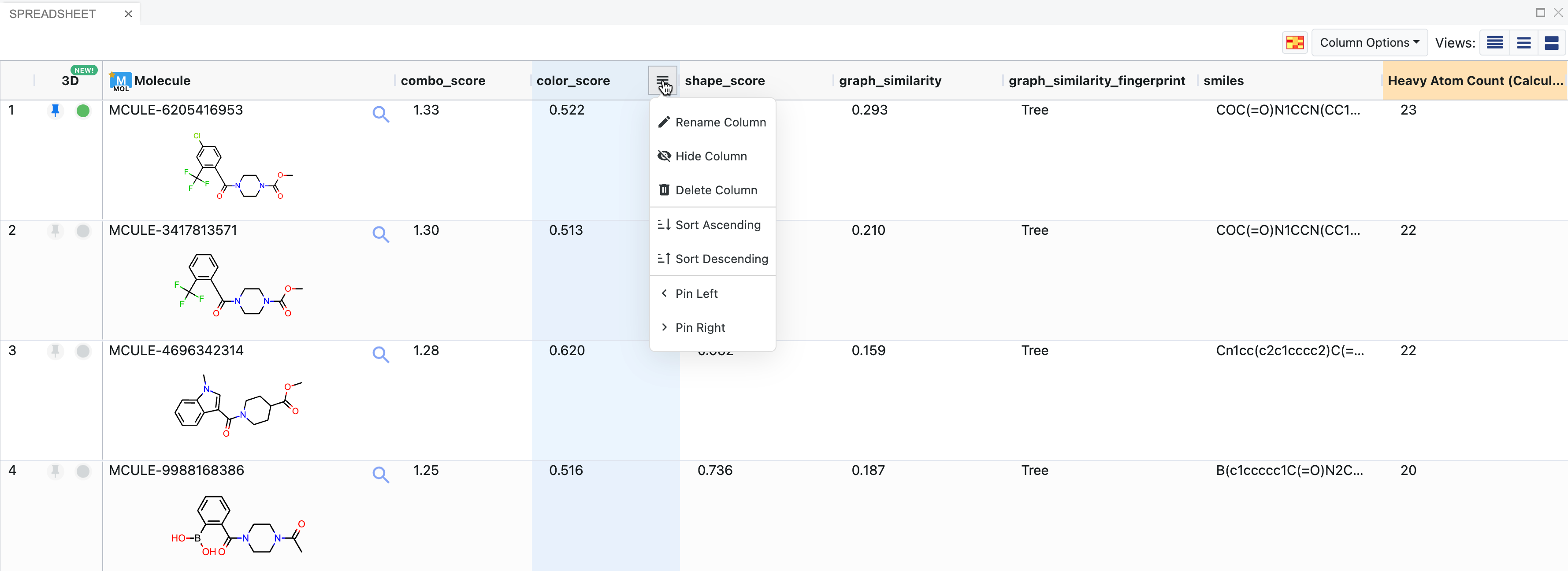
Figure 8. The Spreadsheet. The top molecule is pinned and also activated (green dot) as a visible molecule for 3D. The column menu for the color score is expanded to show the options.
The spreadsheet is populated automatically by fields on the records of a dataset. The fields can come from a variety of sources, including uploaded files (SDF data), floes, or Molecule Search. The spreadsheet can display many types of fields, such as numbers, ranges, molecules, JSON data, and more. SVG images may appear in some fields, such as active site depictions (Figure 9).

Figure 9. Spreadsheet data in the form of SVG images for a bound ligand (6QB) of CDK2 (5K4J) from the SPRUCE - Protein Preparation Floe.
Cells in the Spreadsheet are tethered to points on the plot and to 3D representations in the 3D Viewer. The 3D molecules can be overlaid with the query molecule if desired. In addition, pinned records in the 3D Viewer also are pinned in the spreadsheet and vice versa.
Columns can be resized by dragging the cell border in the heading box to the right or left. Rows can be resized by dragging the border in the row number column up or down. Resizing a row affects all rows, but column resizing is decoupled from other columns.
On the far left of the spreadsheet is a column linked to the 3D Viewer, with icons for pinned records and record visibility; this column appears by default. Each cell showing a molecule includes a magnifying glass which reveals a larger pop-out of the 2D structure. Hovering over a column shows a three-line menu (Figure 8 above) that allows you to sort, rename, hide, or delete columns; columns containing molecules do not include the option to sort. The column can also be pinned to the right or left or set as a record title. To sort columns, you can use this menu to sort ascending, sort descending, or remove sort. It is also possible to sort columns by clicking on the column name: one click for ascending, two clicks for descending, and three clicks to remove the sort. Sorting one column naturally reorders the other columns. Removing the sort returns the spreadsheet cells to the default order. Right-clicking in a cell offers a menu of options to apply to the cell; those with a molecule have additional options to edit the structure in 2D or send it to Molecule Search, as seen in Figure 10.
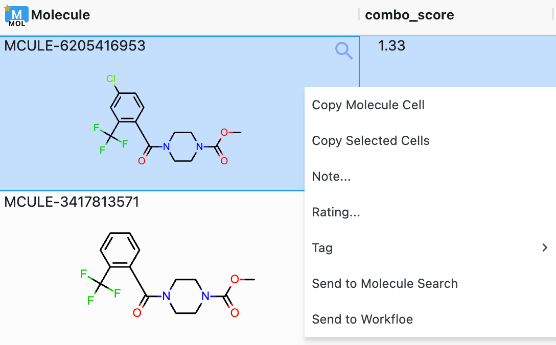
Figure 10. Spreadsheet cells can be manipulated for further use in Orion. To access this menu, right-click in the desired cell.
On the upper left, there are three options for overall spreadsheet appearance: Heatmap, Column Options, and Views. The orange and yellow box allows you to toggle the Heatmap on and off. The colors range from dark orange (highest value) to pale yellow/green (lowest value). ‘Views’ offers compact, normal, and expanded views of the spreadsheet.
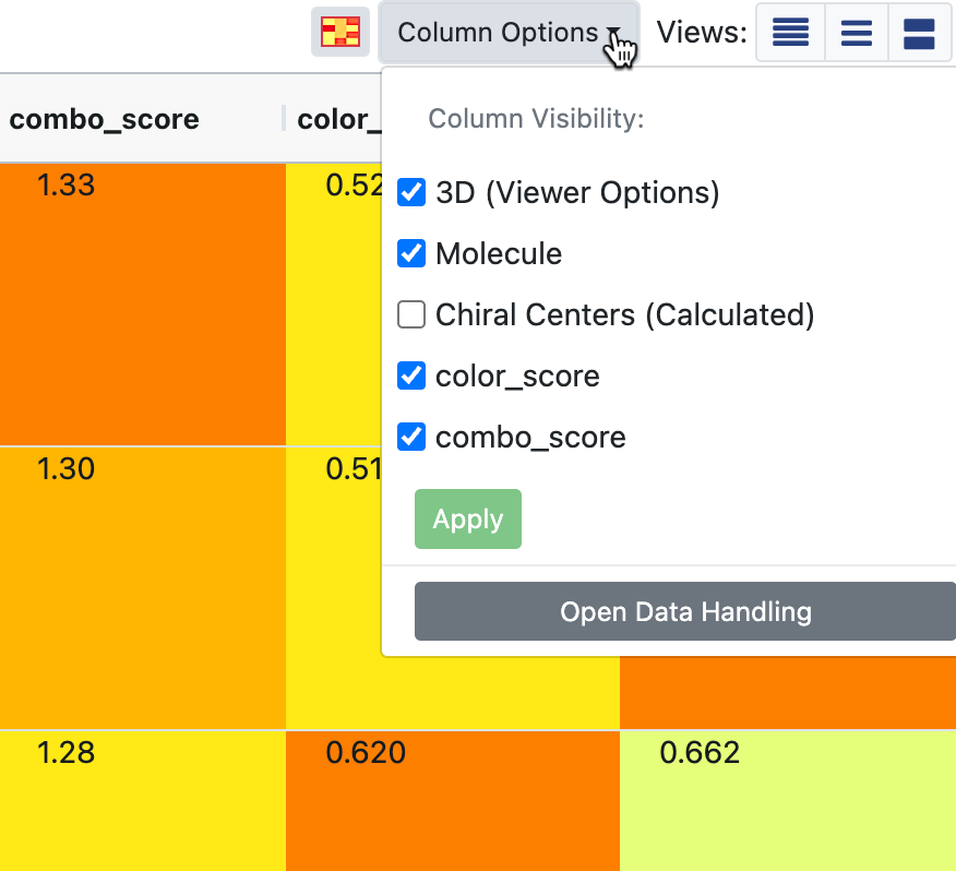
Figure 11. The Column Options drop-down. This image also shows the spreadsheet Heatmap turned on.
The ‘Column Options’ drop-down provides checkboxes for column visibility of all displayed datasets. Select the columns you want and click the “Apply” button. At the bottom of the drop-down is an option to open the Data Handling tool. Note that Data Handling is also accessible from the Active Data Bar. Records occasionally state that the dataset has hidden fields. In this case, hidden fields can be selected through the Data Handling feature. Hiding fields can make data analysis easier in some situations.
Hint
The Data Handling feature allows users to apply column settings to all data columns of the same name for all displayed datasets.
This video shows some basic capabilities of the spreadsheet and the graphing feature.
Plot
The graphing feature can represent data with five different variables, some categorical and some continuous, via the choice of point shapes, size, color, and x and y values. Scatter plots, box plots, histograms, heatmaps, and violin plots are available, where appropriate, for the selected data type(s).
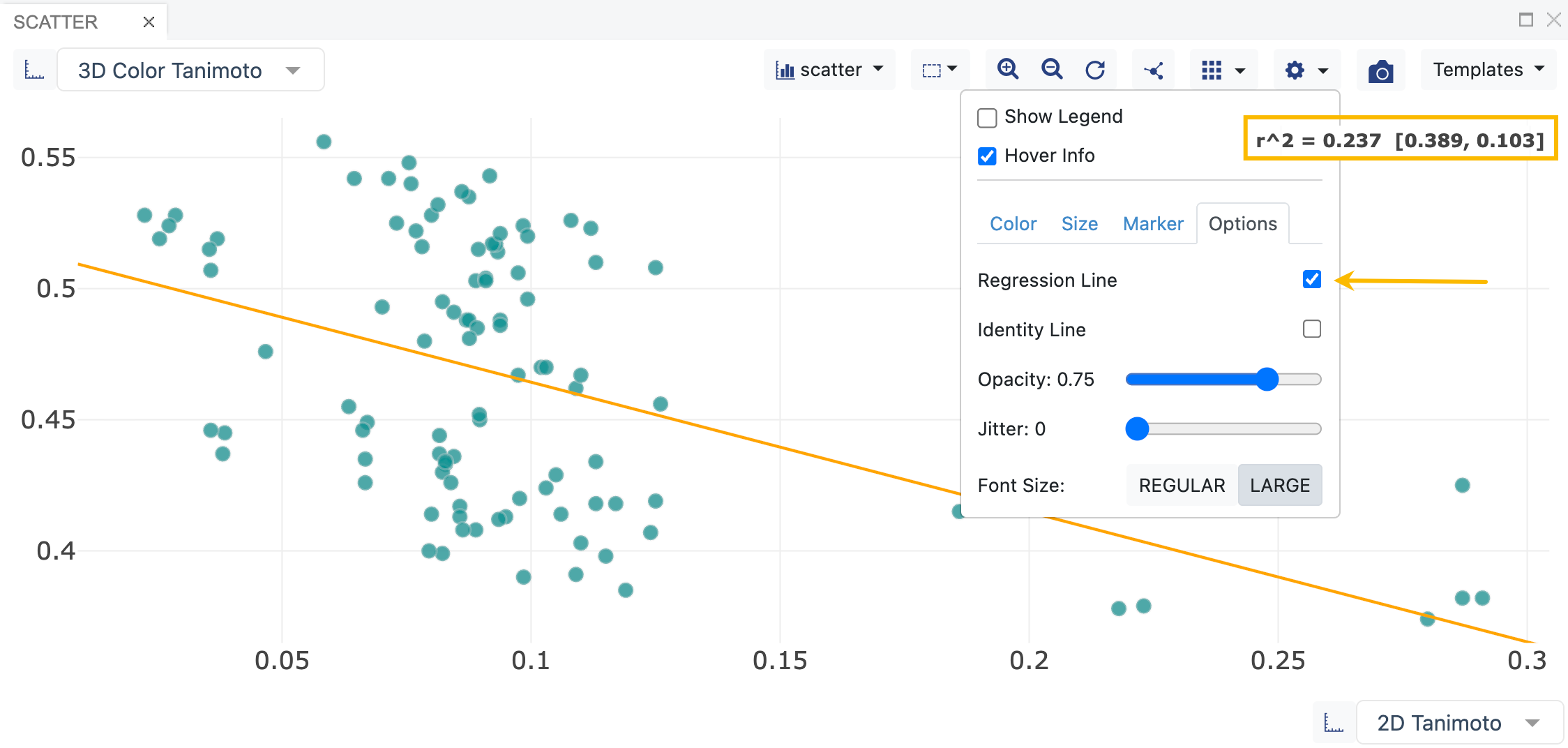
Figure 12. A scatter plot showing how to add a linear regression. Available categories in any dataset can be selected for the axes from the drop-down menus on each axis. Plot type, plot options (such as shown here), and other tools can be found at the top of the graph.
If an active dataset does not display any points on a plot, the legend shows the message “No active data in plot.”
Hovering over a point on a plot shows information about that point, such as the x and y values. The specific information varies depending on the type of plot. Points can be selected by lasso or by point-and-click. Points on the plot are linked to the corresponding cells in the spreadsheet and the depicted 3D structures.
Numerous plot functions are available. The graph can be moved, panned, or reset. Scales can be changed from linear to log forms. Regression lines (with error bars) can be added for scatter plots. Also for scatter plots, more than one dataset can be plotted on the same graph, and the marker style may be customized for each dataset. Box plots contain quartile ranges and other annotations. Multiple graphs can be created. A screenshot of the plot can be taken and downloaded by clicking the camera icon located above the Plot panel.
The Plot Options drop-down (cog icon) provides several ways to customize each plot type. The marker style can be adjusted here, A checkbox allows you to deactivate hover information for each point (default is activated). The regression line for a scatter plot can be added here, and a legend can be added. For scatter plots, multiple datasets can be included on one plot, as shown in the top image in Figure 13. The bottom image shows a drop-down option for the violin and box plot types, in which you can choose the plot’s orientation as auto (default), horizontal, or vertical.
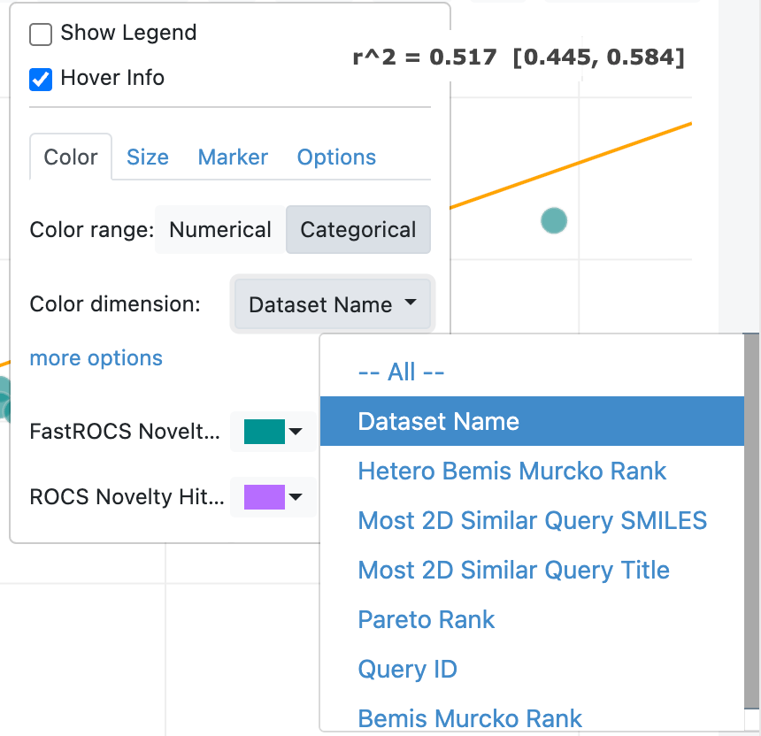
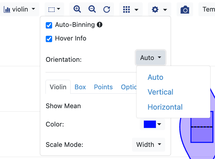
Figure 13. Plot options. The top figure illustrates the use of two datasets in a plot. The bottom figure shows how to choose the orientation of a violin plot.
Data & Columns
This panel offers numerous cheminformatics functions, such as R-group decomposition, property calculation, and a robust multilinear regression feature. Floes that calculate new properties are also available from this panel.
3D Viewer
The 3D Viewer allows the user to interact with and edit molecular structures, examine docking results, perceive protein-ligand interactions, and edit ligands in the context of the active site. Larger panels can be moved, hidden, and resized, which is useful for closer visualization of the 3D window when needed. Also, some features of the 3D Viewer are collapsible: the data tree lists, the 2D depiction of small molecules, and the sequence viewer. Simply click the sideways caret next to the desired feature to collapse or expand it.
3D Data Tree Options
Several options are available for viewing lists of molecular and protein data.
Table 3. 3D Viewer Data Tree Options.
Data Tree Option |
Included Records |
|---|---|
All Data |
All records, organized by dataset |
Pinned Data |
All pinned records |
Focused Data |
Pinned Data + Visible Records + 3D ONLY datasets (selected in Active Datasets drop-down) |
Large Molecules |
Records that include a large molecule (>255 atoms) |
Visible Records |
All records that have something visible in the Viewer |
Visible Objects |
Visible records, but filtered to show only the visible elements |
Note
The Focused Data tree manages the data lists by narrowing down the records to those that are currently being examined. This may offer a cleaner appearance than the All Data tree.
Badges
Each data tree has a list of records. Each record has at least one badge (see Table 4). Badges identify molecules, design units, proteins, grids, surfaces, and components of the DU such as receptors.
The letters come from the field names (such as bl for bound ligand or DG for Density Grid). The colors correspond to the field type. The type is labeled below it. The star on a molecule badge indicates it is a primary molecule.
In general, the badge colors are designated as:
Molecule = blue
DU = green
Surface = purple
Grid = orange
Other = white
They are faded if the field is not shown.
Table 4. Common Badges.
Badge |
Field Name |
|---|---|
d |
designunit |
P |
protein |
L |
ligand |
bl |
bound ligand |
M |
molecule |
OM |
overlay molecule |
Q |
query |
R |
receptor |
IC |
receptor inner contour |
OC |
receptor outer contour |
Cn |
constraints |
DG |
density grid |
DD |
diff density grid |
S |
solvent |
PR |
packing residues |
Ex |
excipients |
For more information on badges and lists in Orion, please see this video.
How to Manipulate Record Information in the Data Trees
Visibility of Records
Note
3D controls for visibility and pinning are linked to the spreadsheet.
The green dot controls visibility of records in the 3D Viewer. To select a record, click the dot to make it green. This can be done either in the data list or in the spreadsheet.
Expand the record using the caret next to its name.
The object may need to be fitted to the Viewer window to be seen. See the Records Menu section below.
Objects in the record that also have a green check will be shown. The green checkmarks are hierarchical, so every parent object must also be checked.
Clicking on a badge in a data tree list can also enable the record in the 3D Viewer.
For small molecules, you can click the molecule badge to show the 2D depiction in the lower left corner if it is not given. For ligands, click the name of the ligand next to the badge to enable the 2D depiction.
For large molecules such as proteins, you can also click the checkmark next to specific aspects of the record (density grid or receptor, for example).
Hovering over the badge will show the structure of any record with “molecule” as a field type (molecules, ligands, etc.).
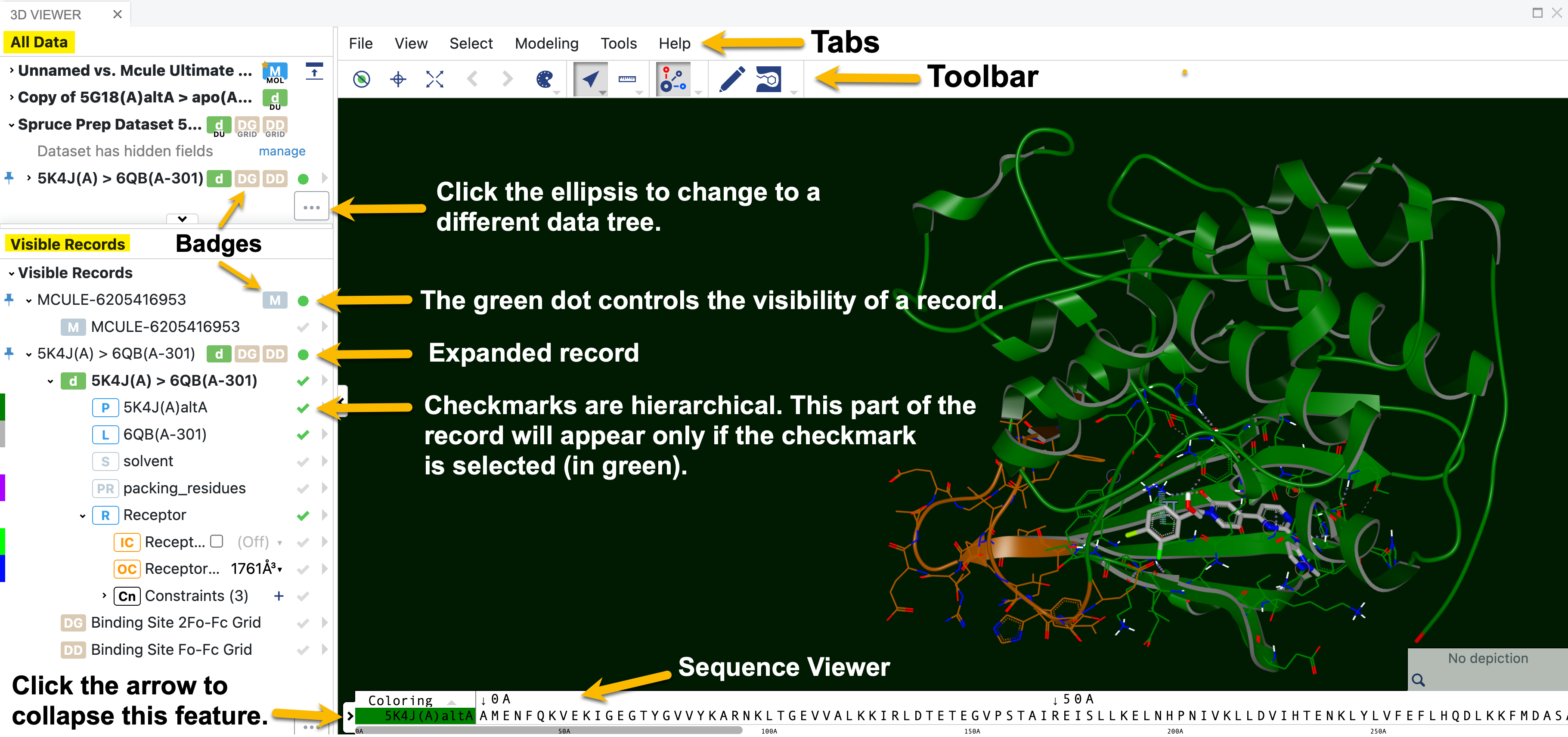
Figure 14. The 3D Viewer labeled to show details of record visibility and general features.
Records can be pinned by clicking the pin next to the record name in either the spreadsheet or the data list. These records populate the Pinned Records data tree in the 3D Viewer and allow you to save them as a separate dataset.
Hovering over the record name reveals a text symbol and star. Notes about the record can be added by clicking on the text symbol. Stars can be added to rate a structure.
Certain actions, such as converting a 2D structure to 3D or editing a molecule, will prompt you to save or discard changes. These options will appear by the record name as disk or refresh icons, respectively.
Convert a 2D Molecule to a 3D Conformer
Molecules in a dataset sometimes appear in 2D rather than 3D. To engage these molecules in three dimensions, it is necessary to convert them to their 3D form. While the molecule can be sent from the spreadsheet to the OMEGA - 3D Conformer Ensemble Generation Floe, it is far easier to generate the 3D coordinates directly in the 3D Modeling layout. You can determine which molecules are depicted in 2D by expanding the molecule file on the left. Molecules in 2D have a red 2D next to the molecule badges, as shown by the yellow arrow in Figure 16. Simply expand the caret, click the three-dot menu, and select Generate Coordinates. A 3D depiction of the molecule will now be available, as shown in the inset. The 3D depiction can either be saved or reverted to the 2D form.
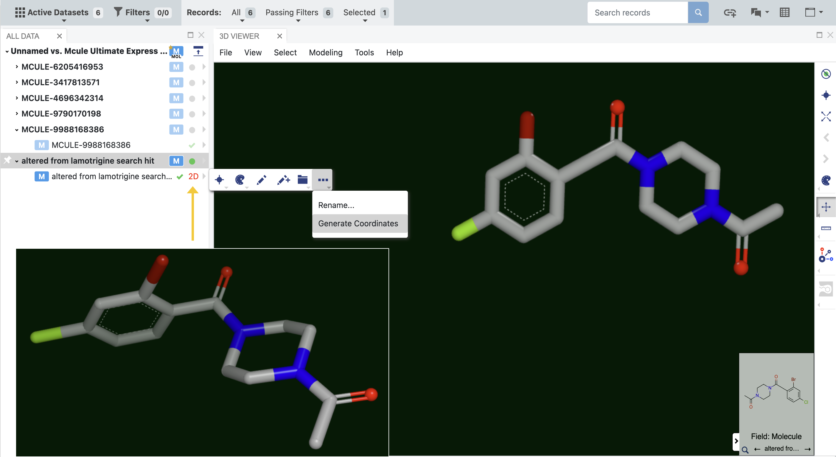
Figure 16. Molecules that are displayed in two dimensions in the 3D Viewer can be converted into 3D structures. The inset shows the generated 3D structure.
Another option for generating 3D coordinates is to edit a structure using the pencil icon in the Toolbar.
Sequence Viewer
Specific residues of a selected protein can be located and selected from a sequence viewer at the bottom of the 3D Viewer. When a residue is clicked, it is highlighted in the 3D window. Conversely, when residues are selected from the 3D Viewer menu, the residues in the sequence viewer will also be highlighted. To collapse the sequence viewer, click the arrow on the left side of the strip. To return it to view, click the arrow on the right side of the window.
Toolbar
Definitions of these tools are included in Table 5.
Table 5. Toolbar Definitions.
Tool Symbol |
Tool Name |
Function |
|---|---|---|
Hide visible objects |
Visible objects are hidden and must be reselected from the data trees |
|
Center viewport |
Center the view on selected atoms or the entire scene |
|
Fit viewport |
Fit the view to selected atoms or the entire scene |
|
Fit previous/next |
Fit to previous or next selected residue |
|
Style |
Style the selected atoms |
|
Switch mouse mode |
Use mouse mode options to move molecules in the Viewer |
|
Measurements |
Use mouse mode to create measurements |
|
Auto-interactions on/off |
Set auto-interactions |
|
Edit molecule |
Edit the selected molecule |
|
Generate binding site |
Generate a binding site using the protein and ligand |
Hide Visible Objects
This button removes all visible records from view. Records must be reselected from the data trees.
Style
As opposed to the Style option accessed from the caret menu of a single record, the Style option in the Toolbar allows for styling the appearance of all records in the 3D Viewer. The dialog box allows you to change styles, colors, labels, and more for all visible objects.
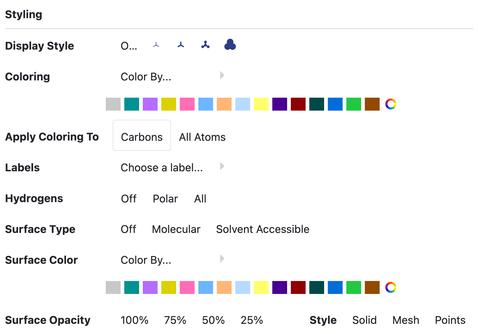
Figure 19. The Style tool dialog box.
Display style affects the appearance of the atoms, such as wireframe and ball-and-stick.
Coloring options allow you to customize structures by element, formal charge, partial charge, residue, chain, and various protein components. Colors can be chosen from a prepared list or via a color wheel, and they can be applied to carbons or to all atoms.
Labels can be applied if desired. Some labels are self-explanatory, such as element or formal charge. Others need additional information:
Index: The index of an atom, a numerical label used to identify one atom from another.
BFactor: The estimated (isotropic) MSD in the atomic position.
Occupancy: The estimated (fractional) population of a particular conformer.
Alt Location: The alternate location of the residue associated with an atom.
Map Idx: The map index of an atom, used to track equivalent atom positions.
Implicit HCount: The number of implicit hydrogens; that is, hydrogen atoms that are not explicitly drawn out but are associated with the parent atom.
Custom: A text box allows you to input a custom label.
Hydrogens can be turned off, or turned on for either polar or all hydrogens.
Proteins can be viewed in ribbon, Cα, or backbone style. Color options are available as above, with similar customizations as above. You can choose to either show or hide waters.
Surface Type can be turned off or set to molecular or solvent accessible views.
Surface Color can be set to curvature, electrostatic, or atom color.
Surface Opacity can also be adjusted.
Style (of the surface) can be set to solid, mesh, or points.
Switch Mouse Mode
This option includes seven different modes to manipulate the 3D Viewer.

Figure 20. The Mouse Mode options.
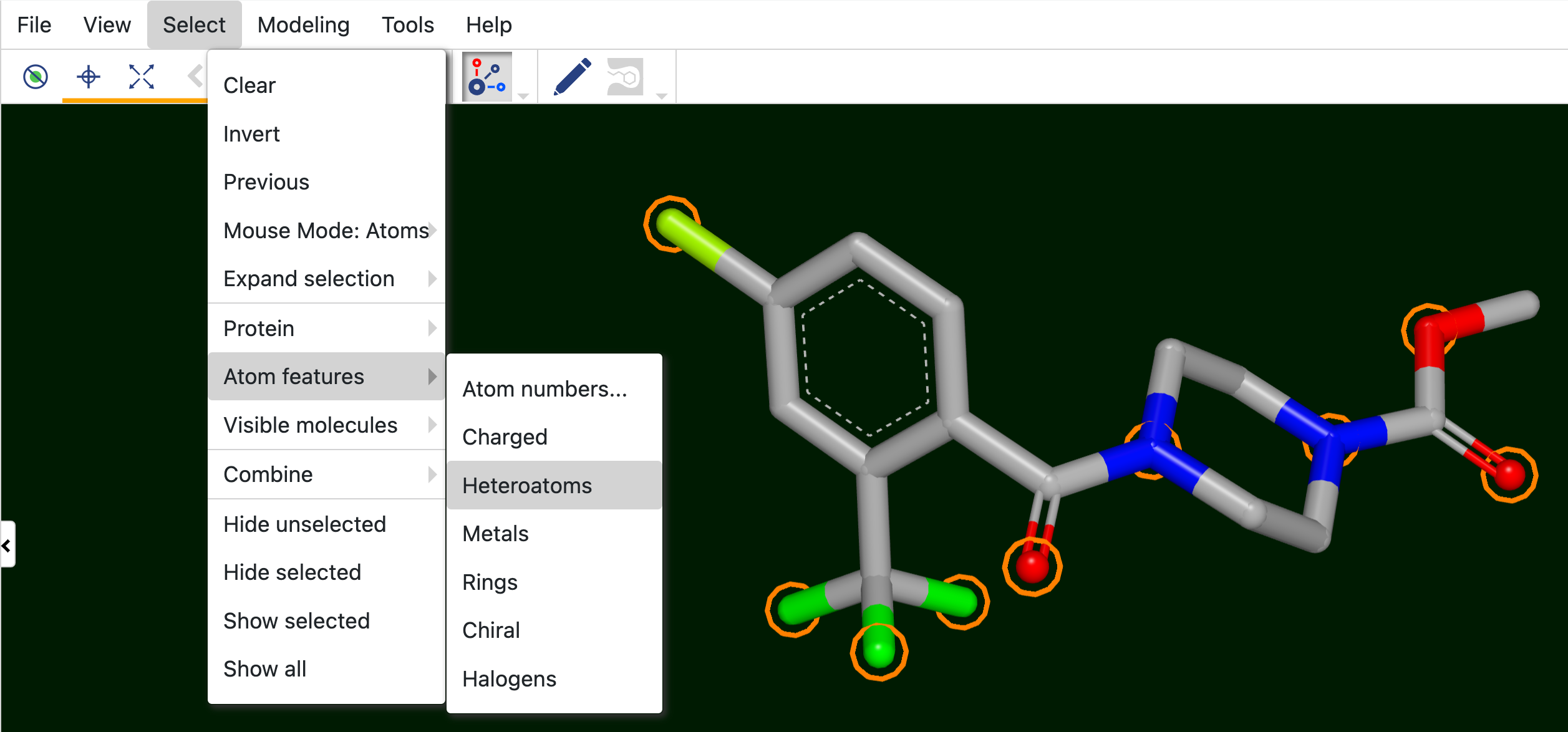
Select allows you to click on atoms or bonds in the structure to highlight them.
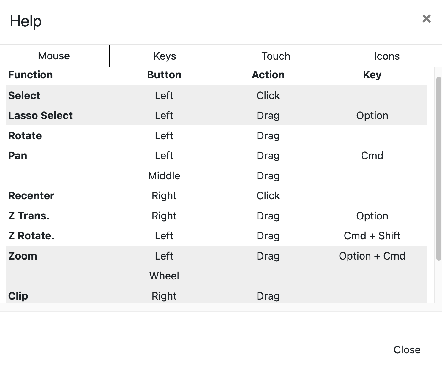
Z rotate allows you to rotate the molecule in the Z-plane only. Cmd+Shift provides a shortcut for this menu option.
Translate allows you to click-and-hold so you can move the entire molecule without rotation. Left click-and-hold plus the Cmd button provides a shortcut.
Zoom allows you to zoom in and out on the structure. The scroll wheel also performs this task.
Z translate moves the scene forwards and backwards, which affects the view relative to the fog and the clipping panes.
Clipping pane mode controls the view. It allows you to change how much of the molecule you can see. Ctrl+hold is a shortcut. If you find that part of your molecule “disappears” into the plane when it is rotated, the clipping pane can be moved farther away.
Lasso Selection highlights a lassoed selection.
Measurements
The mouse can make specific measurements for distance, angle, and torsion. To make these measurements, select the quantity you want to measure. Click on the first atom. Then for distance, click the second atom and the distance (in Å) will appear. For an angle, click three atoms to see the angle. Similarly, for the torsion angle, click four atoms in the molecule.
Viewing Interactions
Interactions between a protein and small molecule can be viewed and selected by using the Viewing Interactions tool. Click on the icon to turn this feature on or off. To select the types of interactions you want to visualize, click the caret. At the top of the pop-up window, the protein name is listed. If more than one large molecule is active in the 3D Viewer, an arrow will appear to the right of the molecule name and a different protein can be selected. Figure 21 shows the interaction options that are available for a given protein and ligand.
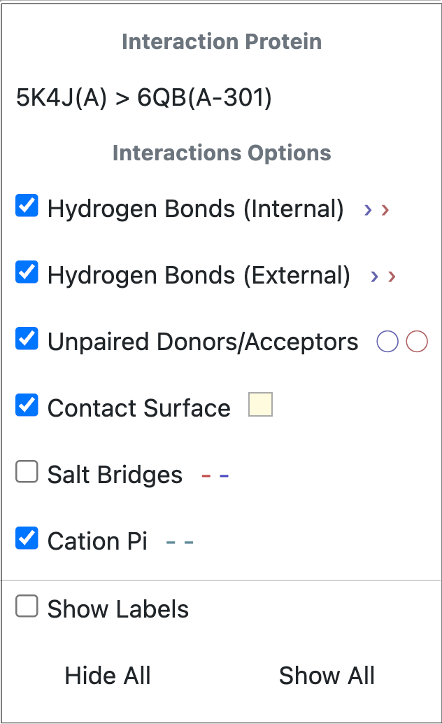
Figure 21. Interaction options for a protein. The features can be selected using the checkboxes. The symbols to the right show how the interaction will appear on the protein.
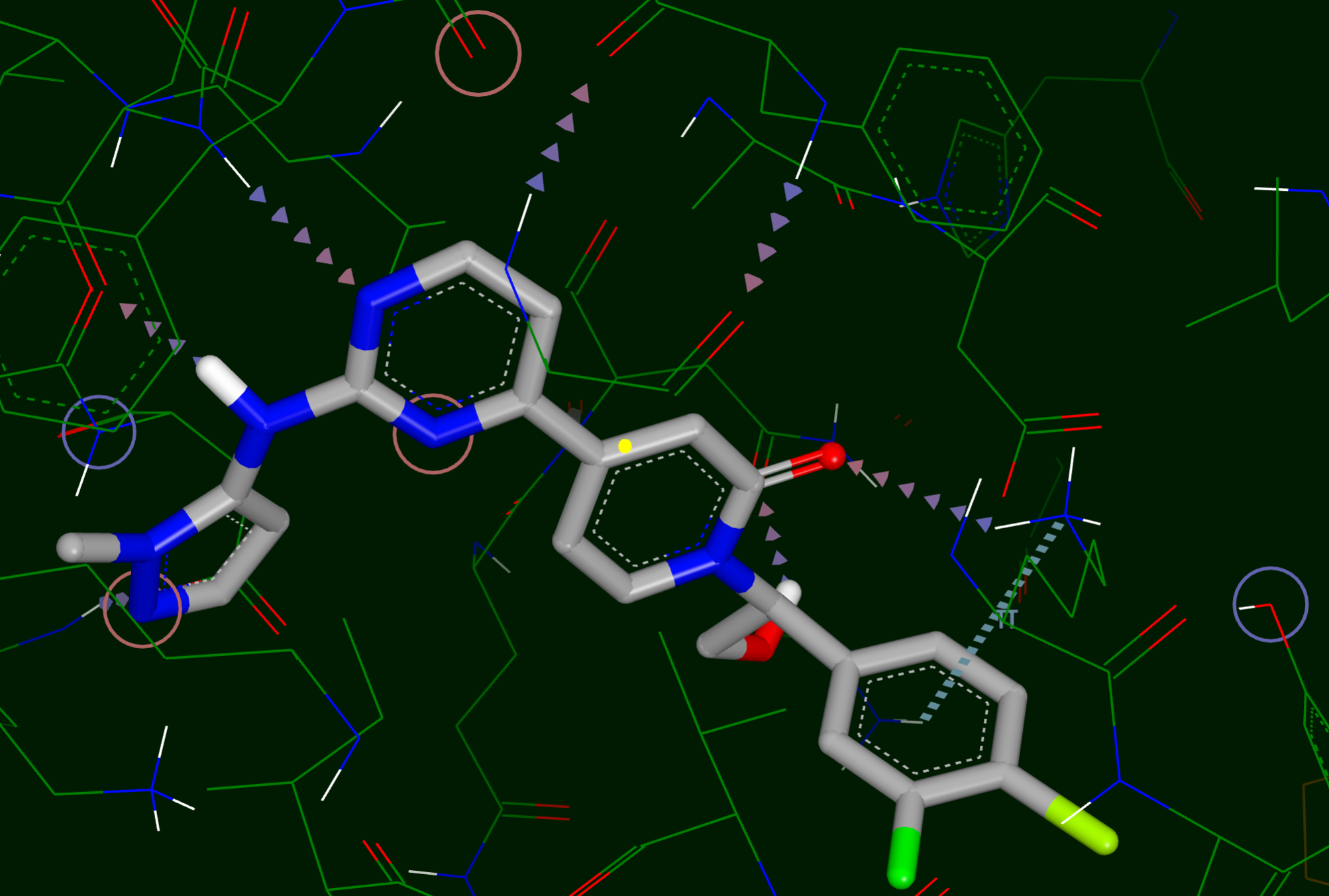
Figure 22. A visualization of the interactions between a ligand and the binding site.
Edit Molecule
Note
Molecules can be edited directly in the 3D Viewer using the pencil icon from the Toolbar.
A structure can be edited using the pencil icon in the Toolbar, and from the side menu for a particular record. Clicking the icon brings up a “Click a molecule to begin editing” prompt. For structures with conformers, a dialog box will ask whether to discard conformers. They must be discarded in order to edit the molecule. After selecting the molecule, an additional toolbar appears to the left, as shown in Figure 23.
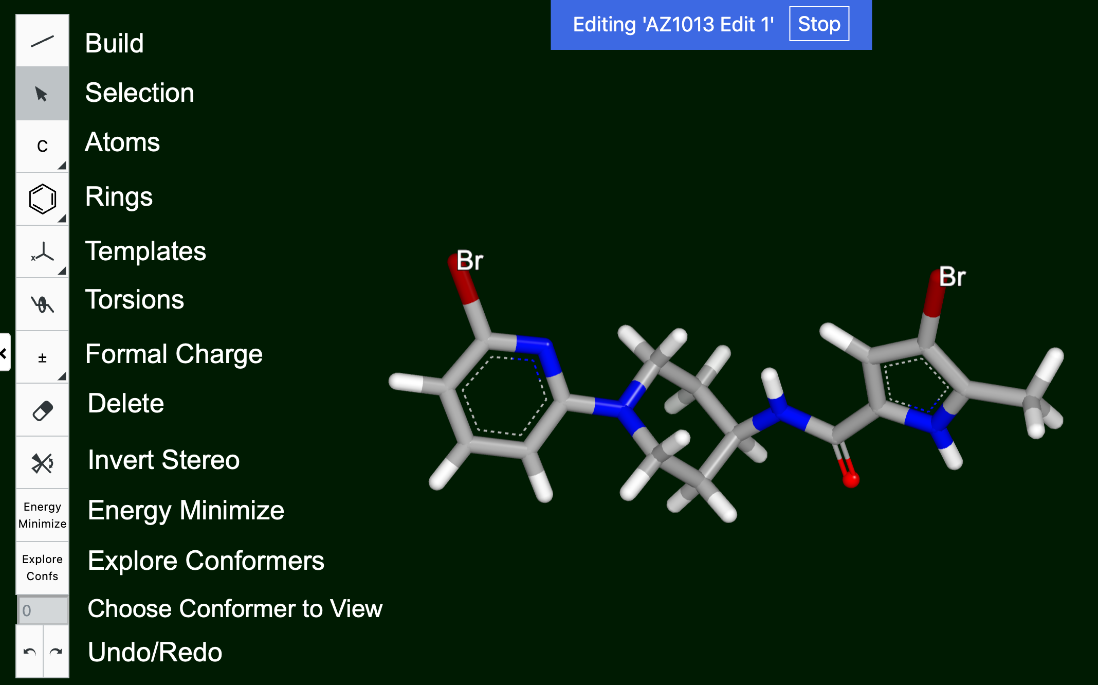
Figure 23. The Edit Molecule toolbar.
Several options are the same as those seen in other UI Sketchers. Others are described below:
Torsions: The torsion angle can be measured by clicking on a rotatable bond. The torsion angle will appear. It can be adjusted using the mouse scroll wheel. Shift+hold gives fine control over the torsion angle, and Cmd+hold changes the part of the molecule that is rotated. If the bond is not rotatable, it will not be highlighted in light green and will not show a torsion angle.
Formal charge: The formal charge can be increased or decreased by 1. Clicking +/- should automatically assign N +1 and C -1.
Invert Stereo switches the stereochemistry around a chiral atom from one enantiomer to another. If a chiral atom is shown on the 2D depiction with a wedge or a dash to represent an atom coming out of or going into the plane, the 2D depiction will reflect changes to the 3D depiction.
Energy Minimize adjusts the structure to the lowest energy configuration.
Explore Confs examines different conformers of the structure. To use this feature, be sure both that the Mouse Mode option under the Select tab is set to atoms and that the ‘Edit Molecule’ toolbar is not on the build or delete buttons. On the Viewer toolbar, choose the lasso option under change mouse mode. Lasso the portion of the molecule you want to explore. For the entire molecule, lasso the entire molecule. Next, click on the box below the “Explore Confs” box and use the up and down arrows to toggle between conformers. The number of conformers (up to 20 conformers) will be listed under the record in the data list to the left. To remove that list of conformers and explore another part of the molecule, click the back arrows at the bottom of the toolbar until the conformer list in the data list goes away.
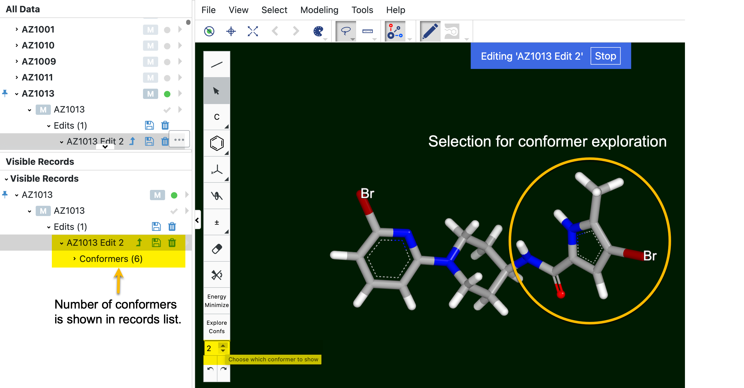
Figure 24. An example of the Explore Confs tool. In this example, a copy of the molecule is being edited. The part of the molecule used to explore conformers is circled in yellow. Compare that part of the molecule to the same area in Figure 23 to see the difference between these two conformers (of six total).
Edit the molecule as desired. When you are finished, click “Stop” above the molecule. The edited structure can be saved or discarded using the icons next to the structure record. Saving the edited molecule reveals a text box with options to overwrite the existing record or save it to an existing or a new dataset.
For a brief demonstration, see this video about Editing Small Molecules.
Create a New Molecule from a Selection
In the course of your investigations, you may want to combine pieces of multiple molecules into one molecule for further investigation through a search or a floe, such as BROOD. Perhaps the end fragments of a hit interact well with a binding site, and it would be helpful to use two fragments to find possible 3D cores. Or you may have molecules or fragments from two different datasets that you would like to combine as a composite molecule. In another case, two promising hits could be merged to find possible combinations of these structures to produce other hits. Alternatively, you may want to extract out a subset of a single molecule, say the binding site of a protein. In any situation, you can create a new molecule file from any set of atoms on the screen.
The All Data tree must be expanded in the records list on the left, or you will not be able to see the New Molecule dataset and record. See Figure 26.
When the desired molecules or fragments are in the 3D Viewer, highlight them, then click “New Molecule” under the Select tab.
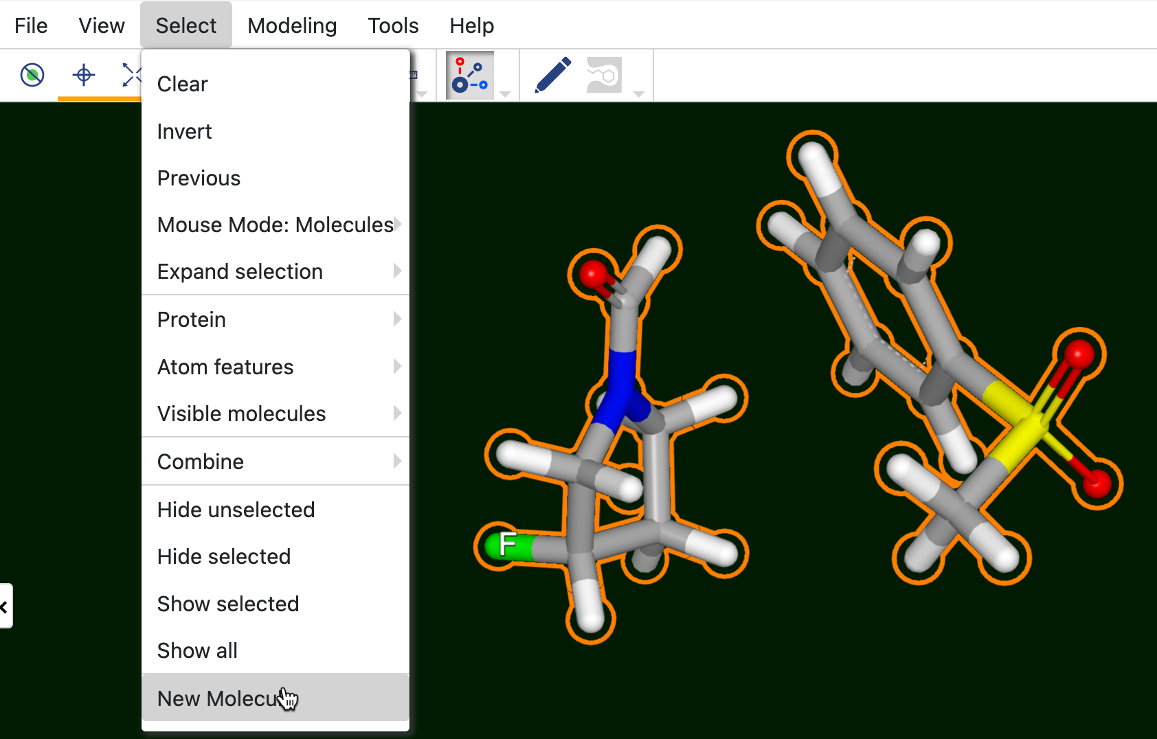
Figure 25. Change the Mouse Mode to Molecules and click a fragment to highlight all. Then click “New Molecule” to create a new molecule file.
You will see a new record named a New Molecules dataset at the top of the All Data tree list. You can rename the “New Molecule from Selection” by clicking the side arrow next to record and then the three dots on the Records Menu.

Figure 26. The New Molecule dataset appears at the top of the All Data tree. You rename the new molecule record as shown here.
To save the new molecule, click the disk symbol next to the New Molecules record. You can choose to make this a new dataset, which will appear as a new record below the other records. Alternatively, choose “More Options” in the Save Molecule modal. This gives you the option to append the new molecule to an existing dataset or to save the new molecule in a new dataset (with the option to specify a path for the dataset). At this point, you can revert to the original record without losing the new (saved) record containing two fragments. You can also remove the New Molecules dataset by clicking the trash can icon.
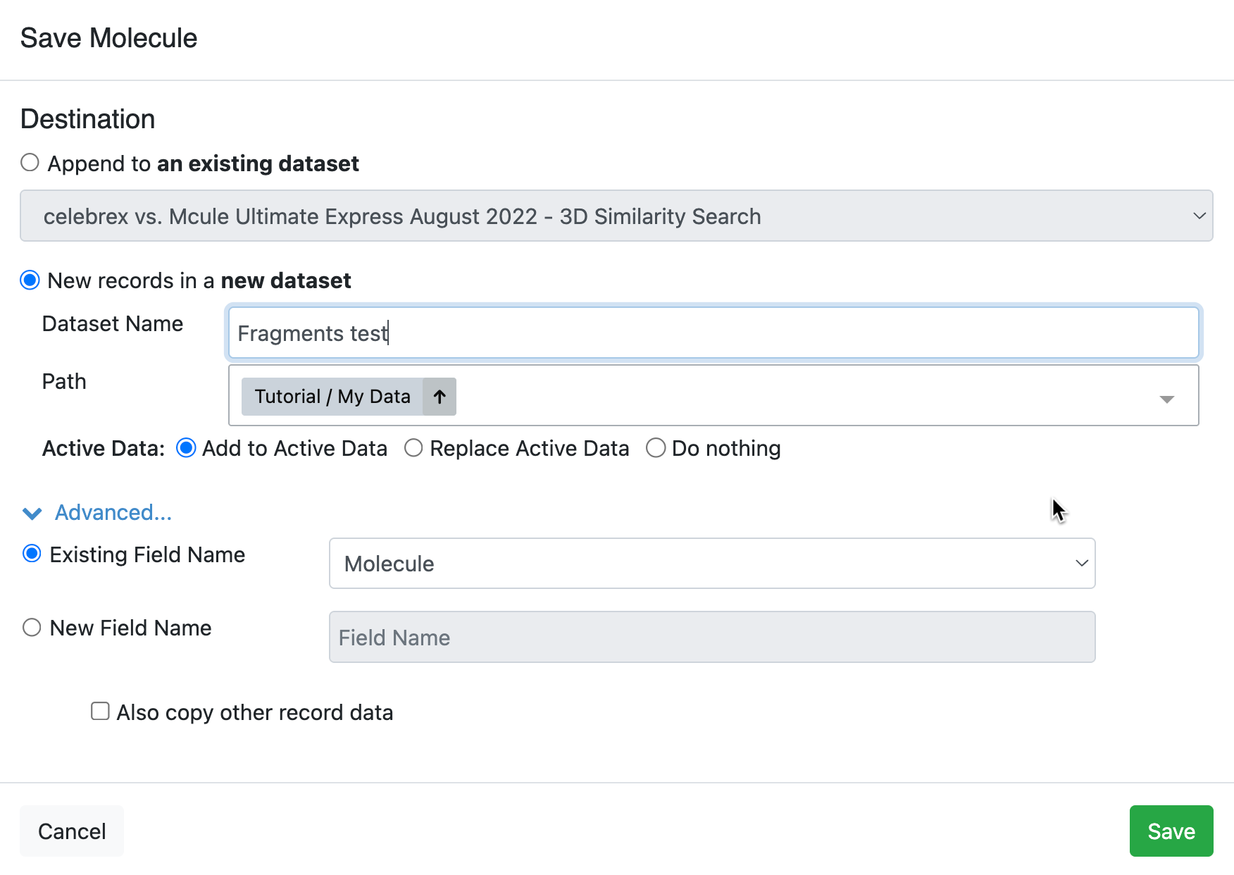
Figure 27. The Save Molecule modal gives options for saving new molecule records.
You can send the new record to a floe or to Molecule Search by right-clicking on its name in the data tree or on the structure in the Spreadsheet.
Binding Site Options
Styling and visualization tools specific to the binding site of a protein and ligand can be accessed with this tool. A binding site is generated by clicking the Binding Site tool. An icon will appear in the records list next to the checkmark for the protein badge; this icon can be used to toggle the binding surface on and off. If more than one ligand or small molecule or more than one large molecule are in the Viewer, a drop-down in the pop-up window allows you to choose which ligand or protein to use. Select how to visualize the binding site by clicking the caret under the Binding Site button.
Figure 28 shows the available options for the binding site. The active site is defined by the distance from the ligand (in Å). Checkboxes allow selections to fit the view to the ligand, create a binding site surface, style the protein, show the ribbon, and show labels. Specific changes can be made with the Style tool. If Style Protein is checked, the active site residue and distant residue styles can again be selected. If it is not, these options are not available, and it is not possible to deselect the Show Ribbon checkbox. After changes are made to the binding site options, a Regenerate button will appear in the pop-up window. Clicking this button will regenerate the binding site with the new parameters.
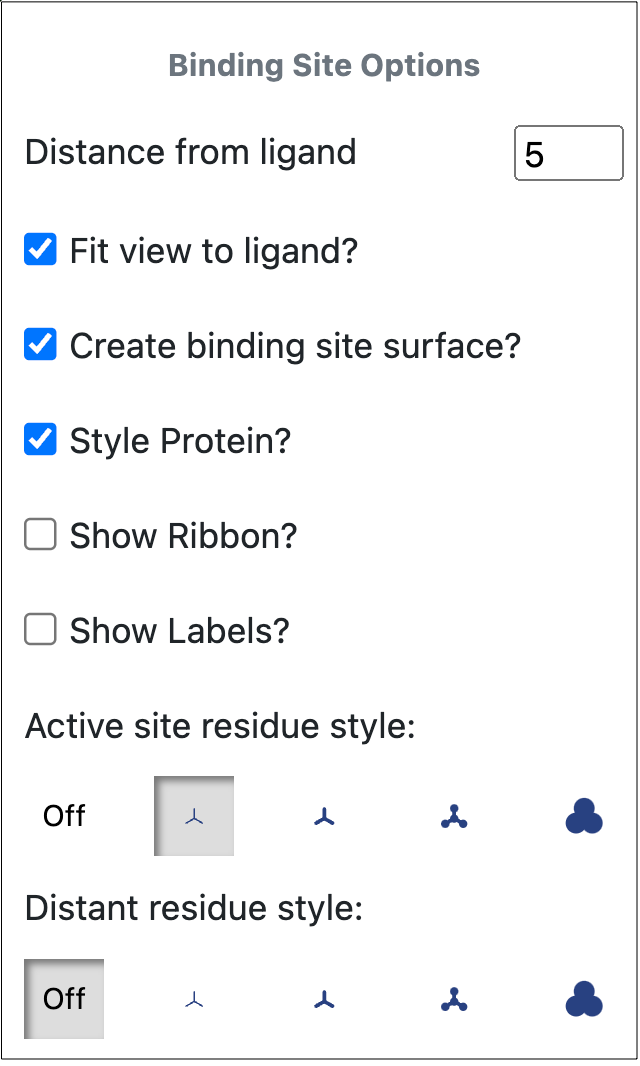
Figure 28. Binding site options from the Toolbar.
Binding site coloration is determined by the electrostatic potential of the protein. Potentials are calculated with OECalculateSurfacePotentials from Spicoli TK. That potential is then used to do a linear gradient such that all values less than -10 are red, blending from red to white between -10 to 0, then blending up to blue at 10.
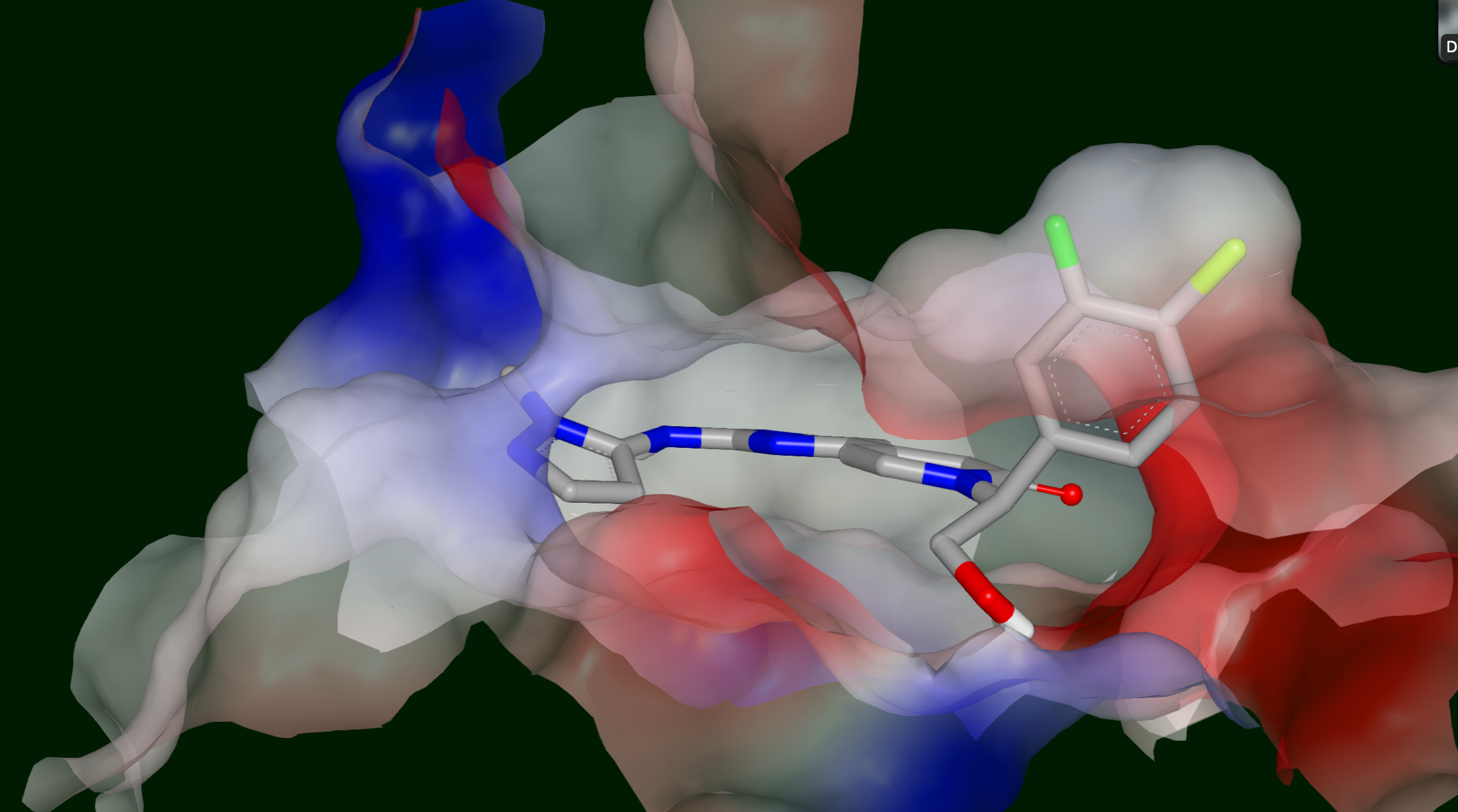
Figure 29. The binding site of CDK2 (5K4J) with a ligand (6QB) after being prepared through Spruce.
Views can be altered using the styling tools (both on the Toolbar and for the individual records), binding site options, interactions options, and clipping pane. The binding site can be viewed with or without the protein or interactions, with receptor inner and outer contours (see Figure 31 for an example), and with different coloration.
Modeling Features
Edit DU Receptor
The Edit DU Receptor feature allows you to modify your receptor grid directly from the 3D Modeling layout. In protein modeling, this is especially useful for docking optimization and analysis.
Edit Receptor allows you to define a box enclosing the active site. The box should enclose the entire region of the active site where heavy atoms of the docking ligand can be placed. Any docked pose with any heavy atom that lies outside the outer contour of the receptor will be rejected.
If a bound ligand has been specified, the default box will automatically surround the bound ligand.
The size of the active site strongly impacts the time and cost of docking. The volume of the outer contour is the most relevant way to measure this size, into which all heavy atoms of docked poses must fit. You can also add constraints to the receptor to reduce the time and cost of docking, although there is a diminishing effect with too many constraints.
To use this tool, choose a design unit (DU), then select Edit DU Receptor on the Modeling drop-down menu.
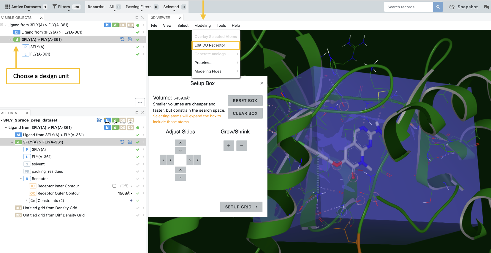
Figure 30. Defining the grid enclosing a receptor.
Once you open the Receptor Editor, you can adjust the size and position of the autogenerated box that defines the confines of the receptor grid. Simply make adjustments with the controls in the Setup Box. The setup box can be adjusted using the Adjust Sides and Grow/Shrink controls. Clicking on a protein residue will also automatically extend the box to enclose the clicked residue. Next, click the “Setup Grid” button for additional options to set the shape site potential and choose whether to generate auto constraints.
The Shape Site Potential is an important factor in the interaction of molecules with proteins. This option defines the inner and outer contours of the receptor. Both contours are always enclosed by the box setup. “Extends toward Protein” means that the contours will extend closer to the protein before extending out into solvent, while “Extends toward Solvent” will cause the reverse to happen. The default, Balanced, is reasonable in most cases.
Finally, click “Build Grid” to build your receptor grid and see details about the contours and constraints. You can save your results at the record or dataset level. The 2023.2 highlights video provides a demonstration.
You can also add a new receptor to a DU if the DU does not have a receptor. The option to add a receptor will only appear if there is no receptor present. Most of the time, this step is not necessary.
From the list of records on the left, you can fine-tune inner and outer contours and constraints as shown in Figure 31. These options are enabled by using the corresponding checkmarks. The size of the contours can be adjusted with slide bars. The inner contour must also be enabled with the checkbox.
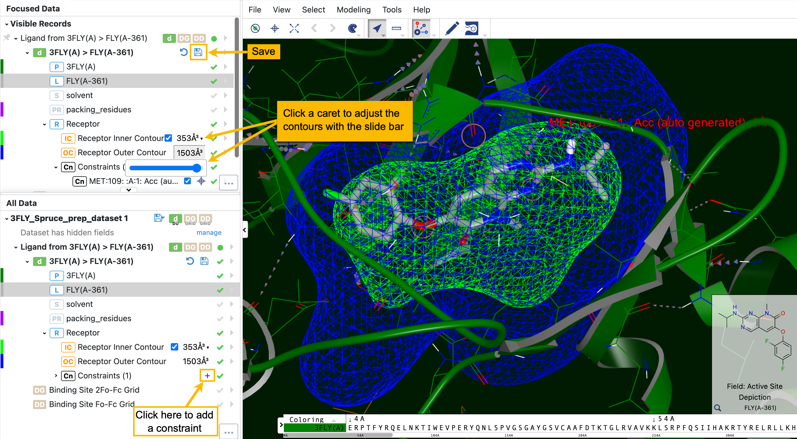
Figure 31. A new constraint can be added with the plus sign. Inner and outer contours can be adjusted with slide bars.
Add and Edit Constraints
Constraints define key interactions that ligands are required to make when docking into the active site. Constraints can ensure that receptor-ligand interactions known to be associated with activity are present in a docked pose. They are optional and user-defined and can be disabled if the constraint is not desired for a particular docking process. If a constraint is enabled, however, any docked pose that does not satisfy the constraint will be rejected. To learn more about constraints, see the theory section of the OEDocking Application.
To add a new constraint, click the plus sign to bring up the “Add a Constraint” box, as shown in Figure 31 above. Two types of constraint can be specified: protein and custom.
Protein constraints are associated with a particular protein atom and are satisfied when a docked pose makes a specific type of interaction with it, such as a hydrogen bond, metal-chelate, or contact with a heavy atom. For a protein constraint, you can select from five constraint types; the default is Hydrogen Bond Acceptor. To add a new constraint, the target symbol in the “Add a Constraint” box must be highlighted, then click on the desired atom to select it.
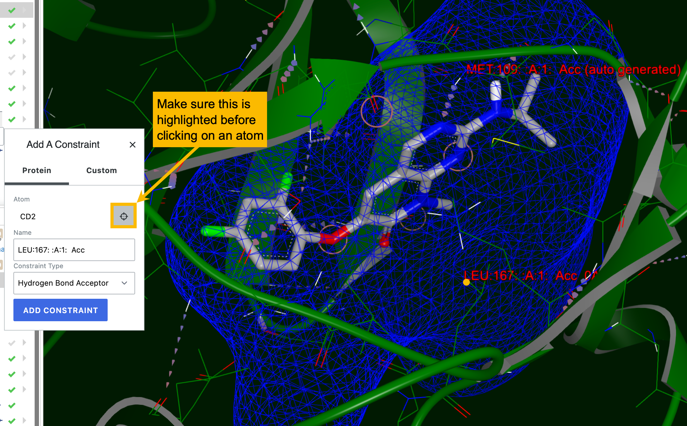
Figure 32. Adding a protein constraint.
Custom constraints require both a sphere or spheres within the active site and one or more SMARTS patterns. Custom constraints are satisfied when a heavy atom of a docked pose falls within a sphere if no specific SMARTS pattern is supplied, or when an atom on the docked pose matching one of the SMARTS patterns falls within a sphere.
To add a custom constraint, choose the “Custom” option to add a SMARTS pattern. You can enter “*” for any atom, a specific atom, or a full SMARTS pattern. The SMARTS box will indicate whether an entry is a valid SMARTS pattern or not. Then click the “+” sign next to the Spheres box and select an atom on a residue. A sphere will appear to define the constraint. Custom constraints allow you to change the size and location of the constraint sphere; they do not need to remain on a particular residue. To add another custom constraint, add the atom or SMARTS on a separate line, click the plus sign, then select the desired atom. You can switch between spheres using the drop-down. Please note that the cursor must be on the SMARTS pattern you want before clicking the plus button to add a sphere. Click the blue “Add Constraint” button to save the new constraint(s). In the records list, click the disk icon to save the DU, or click the revert icon to dispose of the changes.
In the UI, the default sphere size for a custom constraint is 1 Å. The sphere size appears next to the sphere and can be adjusted. You can also shift the position of the sphere using the arrows under Custom Constraints.
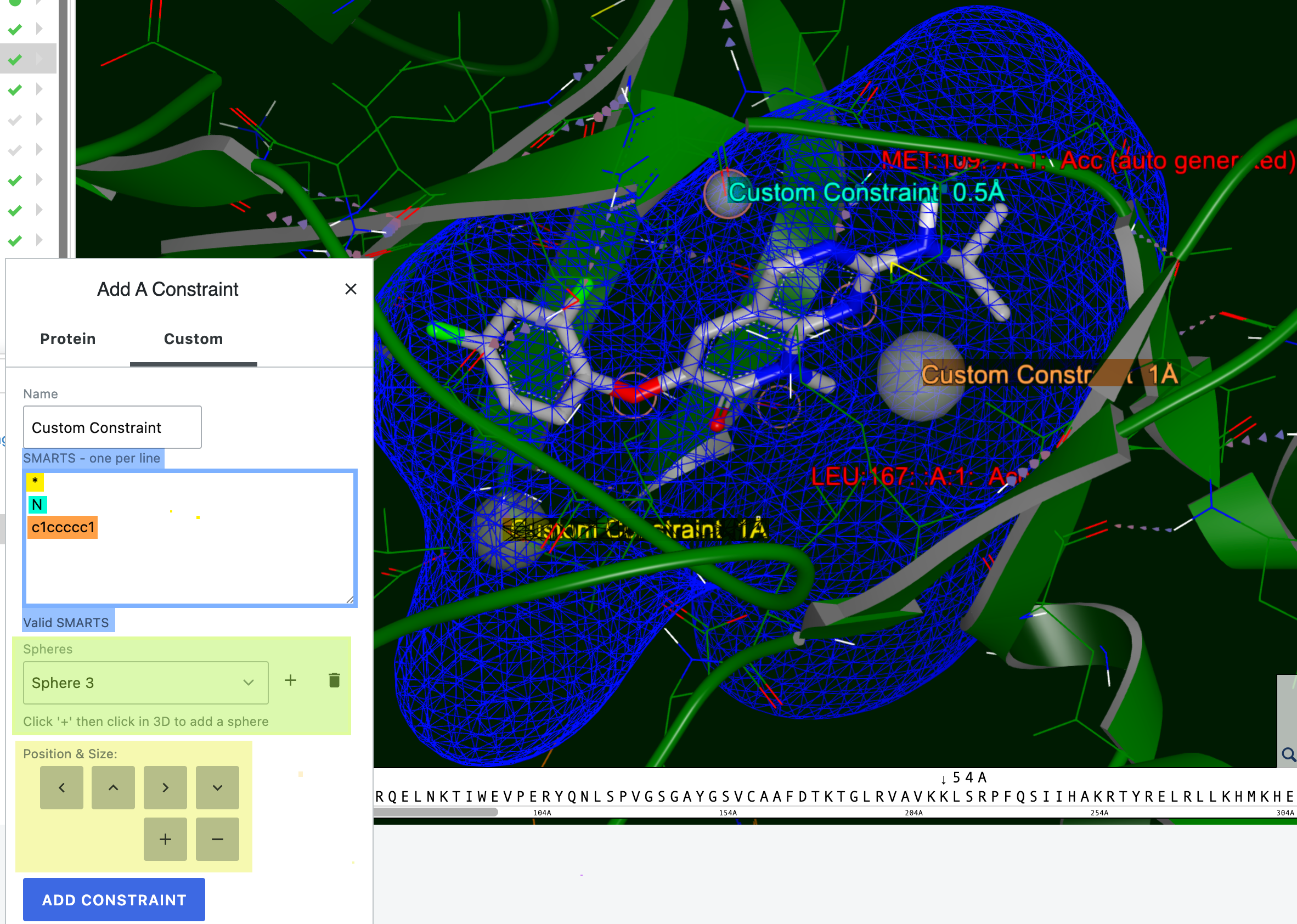
Figure 33. Adding custom constraints. Three were added in the blue box, shown in yellow (* for any atom), teal (N, a single atom), and orange (SMARTS pattern). An alert for an invalid SMARTS pattern will appear below the box. Spheres can be added or deleted in the green highlighted box. The position and size can be changed in the highlighted yellow box. The size of the teal constraint was decreased to 0.5 Å. The orange custom constraint has been moved off of its original position on a residue.
To edit a constraint, click the arrow next to it to bring up the records menu. Clicking the ellipsis will bring up options to either edit or delete the constraint. For protein constraints, be sure the target symbol is highlighted and select the atom where you want to move the constraint. For custom constraints, select the sphere you want to edit and edit as needed. You can also add another custom constraint.

Figure 34. The side menu to edit or delete a menu.
Features for enabling and modifying constraints are covered in the 2023.1 video.
Generate Analogs
This tool provides a way to quickly generate possible 3D conformers of small molecules. It takes a molecular core and adds R groups to produce analogs.
Note
This tool is meant to find quick ideas to test. It is not all-encompassing. For a full investigation using generative chemistry, we suggest using the Generative Structure Floe Site Selection Floe. For more questions or assistance, please email OpenEye Customer Support at support@eyesopen.com.
Four methods are used to generate analogs. For more details regarding how analogs are generated, please see the Generative Design Floes.
The Near Fragments method follows the parameters and methodology of the “Graft” method; new analogs are 60–80% identical to the original molecule.
The Matched Molecule Pairs method follows the parameters and methodology of the “MMP” method.
The Sidechain Exploration method follows the parameters and methodology for the “Sprout” method, but it explores new chemical matter without any notion of reagent selection or synthetic accessibility.
The Reagents method is a non-exhaustive, quick method using four small libraries of reagents—Primary Amines, Carboxylic Acids, Aryl Halides, and Suzuki Boron—to be reacted against a user-defined portion of the original molecule. Please note that this method does not require specific chemistry to be present but instead relies on the user to determine appropriate connections for their application.
To use this tool, activate a structure for which to generate analogs. Choose a method and the structure will be displayed in a pop-up window. You must lasso a selected fragment. Click the “Use selected fragment as input” button. A set of analogs will be displayed in a separate window and can be selected as desired.
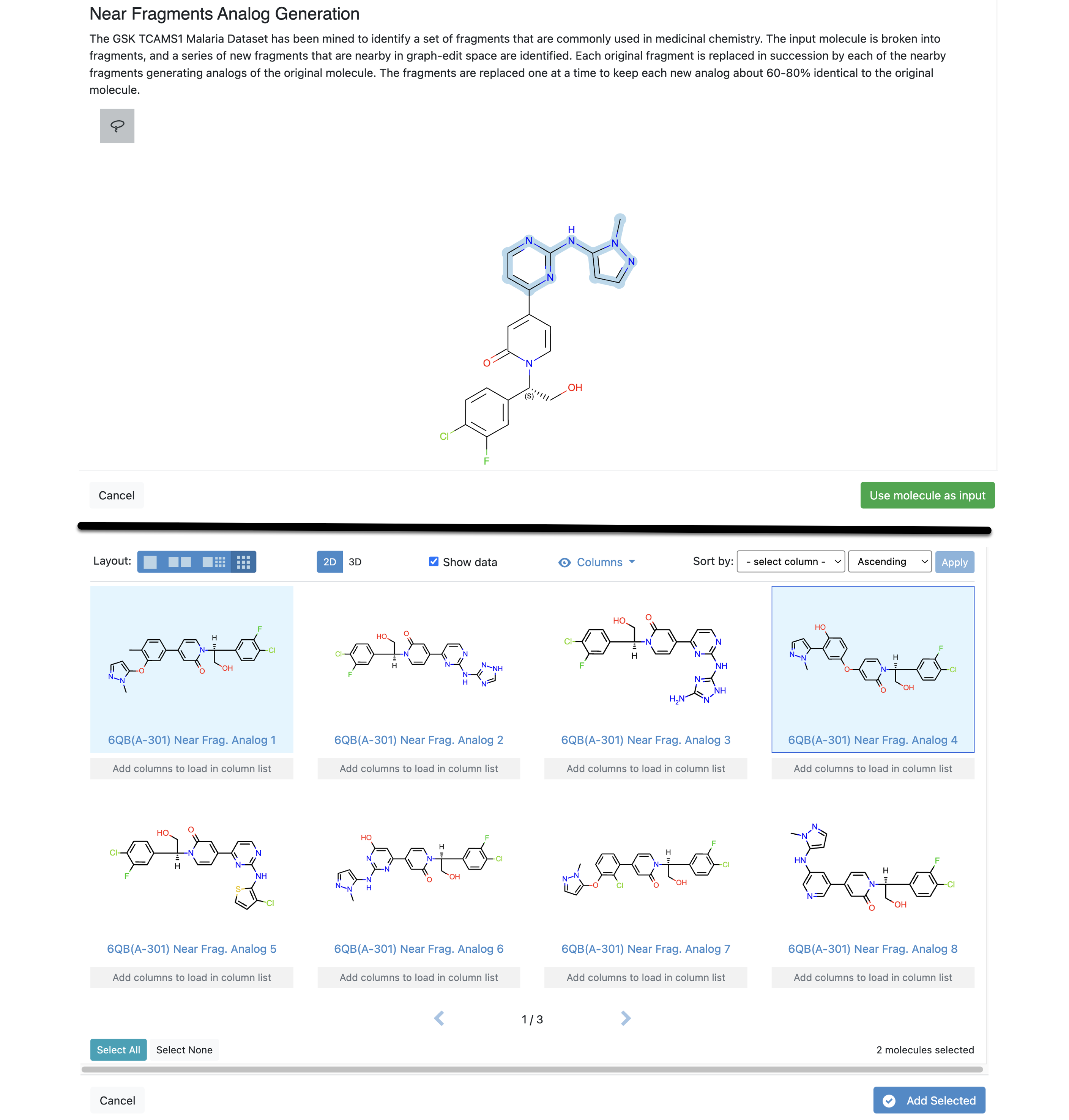
Figure 35. Using the Near Fragments option of the Generate Analogs tool. The top image shows the selected fragment for analog generation. The lower image shows the results. They can be sorted by data fields (columns), such as acceptors or molecular weight, and viewed in 2D or 3D.
Protein Modeling
The Proteins option under the Modeling tab includes several methods for editing large molecules. From the Proteins option, rotamer and histidine states can be changed, residues can be mutated, partial residues can be identified, terminal residues can be capped and converted, and protonation states can be changed. Note that making any changes will remove receptor features.
Change Rotamer States: To change a rotamer state for a residue, select a residue, then select the Change Rotamer States tool. Changing the rotamer state will remove receptor features. To modify the rotamer state for the selected residue, use the arrows in the upper right side of the Viewer window. Once the preferred orientation is found, click the checkmark, or click the red X to cancel the change and return to the original orientation. The original state can also be reached by clicking the refresh button by the record name, or the new state can be saved by selecting the disk icon.
Change Histidine States: This procedure is like that of changing rotamer states. A histidine residue must be selected. This feature can be especially helpful to change protonation in the binding site.
Mutate Residue: To mutate a residue, select a single residue and click the Mutate Residue option. A pop-up window will appear with a table of residue options, or a residue’s code or abbreviated letter can be entered.
One action would be to mutate the residue, then rotate it to optimize fit and interactions in the binding site.
Because mutations can change the binding affinity, this tool can be used to test the effects of different residues in the binding site.
Another use is if you want to use the wild (nonmutated or canonical) form of the protein that matches the crystal data.
Generally, the mutated version is what will be used in analysis. Posit can be used with mutated versions of proteins to give possible poses of ligands. This is useful in testing against known mutations.
Identify Partial Residues: This tool corrects residues when they are missing from the protein sequence. This is important because some downstream floes, such as Molecular Dynamics floes, will fail with partial residues.
Sometimes partial residues are outputted from the SPRUCE - Protein Preparation Floe. The Floe Report will state that the design unit contains “partial side chains.” The Spruce TK theory section discusses why Spruce sometimes cannot build side chains to prepare residues. This typically indicates that manual manipulation is required because the input file may not have enough data to give an optimal residue orientation. Select Identify Partial Residues, and if the record contains partial residues, the first residue will be highlighted, and manipulation options will appear in the top right-hand corner of the 3D Viewer. The arrows toggle between different partial residues in the structure. The Fix button will grow and build the missing side chain atoms. Click the checkmark when the partial residues are fixed or click the red X to cancel and return to the original state.
Example: The structure 1BRS was used in the Spruce - Protein Preparation Floe. The Floe Report includes the following information.
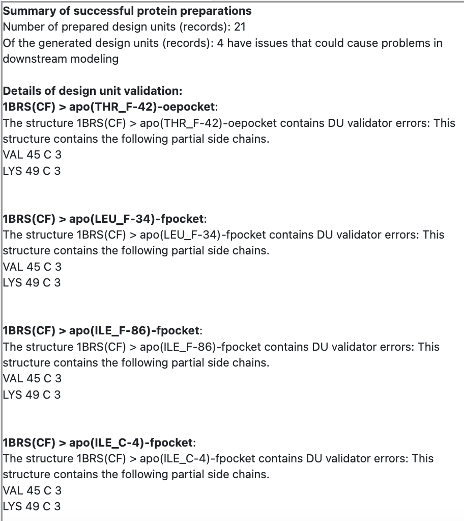
Figure 36. The Floe Report from the Spruce - Protein Preparation Floe.
These partial residues in the structure must be fixed in order to run successful floes downstream. Choose Identify Partial Residues to manually build these missing side chains. Figure 37 shows the window that appears with the selection of this tool.
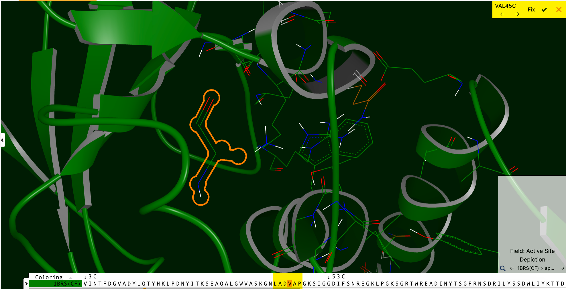
Figure 37. Valine 45 partial residue to be fixed. You can toggle through options with the arrows at the top left. To fix the residue, click “Fix” and either accept the change by clicking the checkmark or revert it by clicking the X. Note that the residue is also highlighted in the Sequence Viewer below.
When you select the residue to be fixed with the checkmark, an information box will ask whether you want to remove receptor features. Choose Continue to build the side chain. The fixed residue will now be highlighted, as seen in Figure 38.
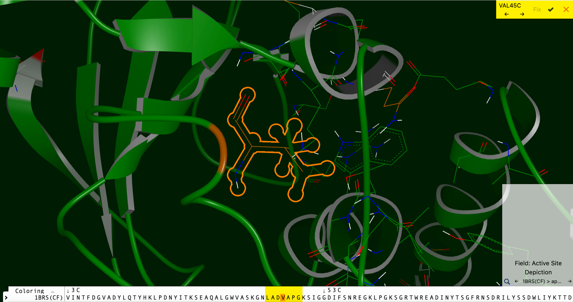
Figure 38. Residue with newly built side chain.
Accept or reject the change in the box at the upper right, then revert or save it using the revert or save buttons in the record list on the left.
Note
When a partial residue is fixed in the Orion UI, clashes may not be taken into consideration, and you may not be able to visualize steric clashes outside the binding site.
For reference, an example of a clash within the binding site is shown in Figure 39.
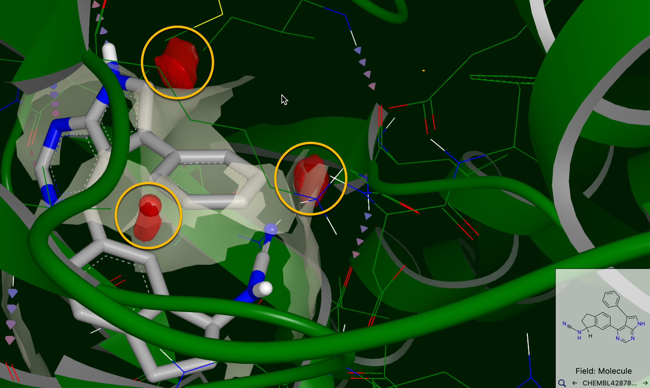
Figure 39. Clashes between TYK2 (PDB ID: 4GIH) and the ligand ChEMBL4287845. Clashes are shown in red and circled in yellow.
Cap and Convert Terminal Residues: This option identifies terminal residues that are not capped. It is described in the Spruce TK OECapTermini function documentation. The arrows toggle between different terminal residues. Clicking the Cap Term button adds an acetyl or N-methyl group, depending on whether the cap is an N- or C- terminal, respectively. The Conv Term button converts the selected residue into a terminal residue capping group. Once the preferred capping is found, click the checkmark, or click the red X to cancel the change and return to the original state.
Protonation: Most biomolecular structures have been generated with either no explicit hydrogens or only polar hydrogens. However, it may be necessary to explicitly represent and position all atoms to make appropriate hydrogen bonds. This tool allows the optimization of hydrogen bonds. As part of this tool, frozen heavy atoms can be selected and selected hydrogens for heavy atoms can be frozen or unfrozen. Frozen atoms are fixed so they do not move during the optimization process. More information on these parameters can be found in the SZYBKI application or the Spruce TK Protein Placement and Optimization section.
Sample Uses of the 3D & Analyze Page
The 3D & Analyze page can be used throughout all stages of data analysis. Here are some examples.
Use the Import Biomolecule tool under the File tab in the 3D Viewer to load a PDB structure. A good example would be 1BRS, as it contains partial residues but does not have a ligand. Fix the partial residues to make the protein suitable for modeling. If desired, you can change the rotamer states or mutate residues as well.
Run the SPRUCE - Protein Preparation Floe. Check the Floe Report and use the 3D Viewer to fix any errors to generate prepared proteins that are ready for a viable MD floe run or other downstream purposes.
Use Edit DU Receptor to move or change a binding site. This could be useful when you have turned on the Enumerate Pockets parameter in the SPRUCE - Protein Preparation Floe. This parameter enables the floe to enumerate multiple binding sites on the protein. The floe can use the Site Residue Entry parameter to do this automatically, but Edit DU Receptor allows you to control this process.
Visualize the results from the OEDocking - Dock into an Active Site for Virtual Screening Floe: a dataset of ligands that are prepared for docking.
Evaluate the output from the Protein Sequence to AI Folded Structure Prediction Floe.
Evaluate the output from a SiteHopper floe.
Evaluate the output from a Cryptic Pocket Detection floe.
The Spruce tutorial gives an excellent example of using the capabilities of the 3D Analyze page to examine and manipulate data.

