Example Commands

Conformer free energies

The default calculation type in free form is -calc conf, so this is what it will run if no -calc option is specified. However, in the following examples we will specify this calculation type explicitly. The two main types of conformer free energy calculations are 1) when the input 3D structure is not known or not of special significance, and 2) when there is one or more input 3D structure(s) we would like to track, e.g. if they are believed to be bioactive conformers. In the latter case, -track is specified, and FREEFORM reports specifically on the global and local strain energies for these conformers.

Note

The numbers and values in the examples below are just for illustration and can change as we improve the applications.

Example 1

Let us begin with case 1 above: when the input 3D structure is not known or not of special significance. In this example the input is the SMILES string for Januvia in file januvia.smi:

(Fc1cc(c(F)cc1F)C[C@@H]([NH3+])CC(=O)N3Cc2nnc(n2CC3)C(F)(F)F)

The command is:

prompt> freeform -calc conf -in januvia.smi -prefix januvia.pfn

This produces five output files:

januvia.pfn.pdf: the results report summarizing key results for each molecule in the run.

januvia.pfn.log: the log file of per-molecule results. This also shows the progress of the calculation if it is taking a long time, for example if the run has to minimize a conformer ensemble containing 20000 conformers (this can take over half an hour).

januvia.pfn.csv: the csv file of per-conformer results (energies, entropies, and free energies)

januvia.pfn.oeb: the file of all the final minima for the molecule.

januvia.pfn.param: all the input parameters of the calculation are written here.

Let us first look at an example of a results report in file januvia.pfn.pdf, shown below.

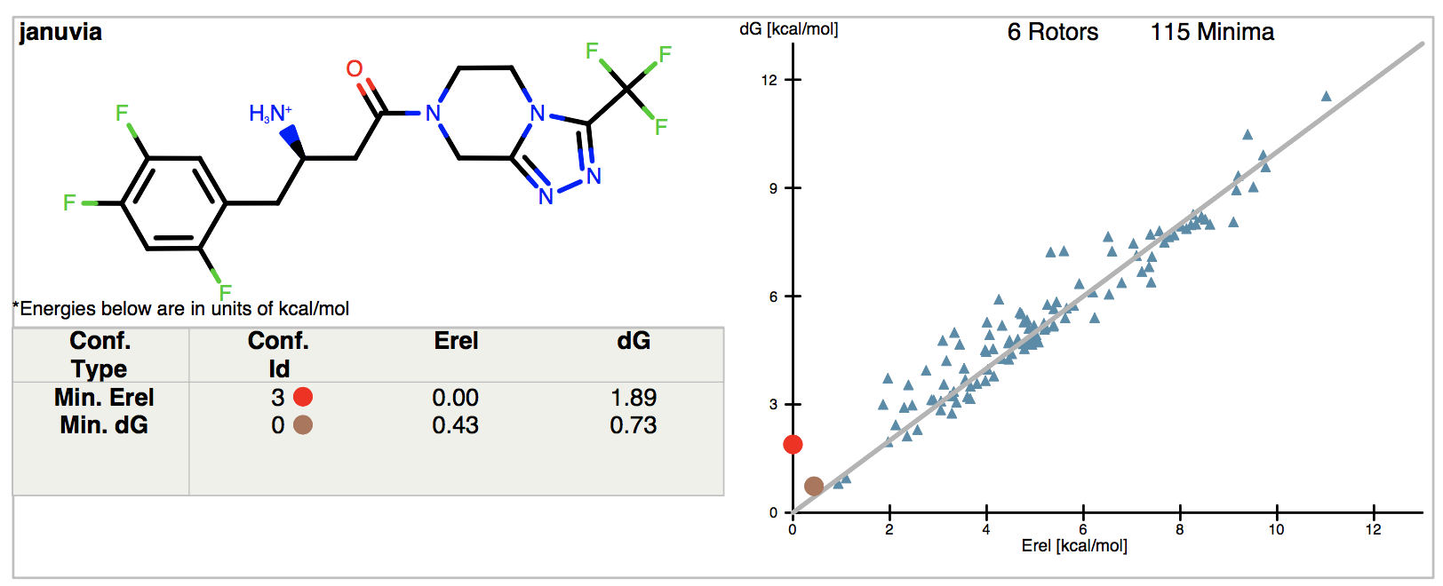
Results report from Januvia SMILES input

A 2-D depiction of the molecule is given in the upper left, and underneath is a table with two entries giving the relative energies (E(MMFF) + E(solv)) and conformer free energies (including entropy) for the relative energy (Erel) and free energy (dG) minimum conformations. All the energy units in freeform are in kcal/mol. The strain information (Local Strain and Global Strain) is empty in this example. The graph on the right-hand side shows the conformer free energy versus the relative energy for all the conformers produced in the calculation for the unbound ensemble. At the top of the graph we note the number of rotors (rotatable bonds) sampled in the conformation generation for this molecule (six), and the number of unique minimal in the entropy calculation for this molecule (188 in this example). The red dot on the graph corresponds to the relative energy minimum (see the conformer also labeled with a red dot in the logfile table; the conformer id can be used to reference it in the .oeb file, and in the .csv file), And we can see from the table and the graph that while it is the global energy minimum in terms of enthalpy, it would cost the dG amount in conformer free energy to select this conformer from the aqueous free-ligand ensemble. In contrast, the Min dG conformer has the lowest free energy (corresponding to the brown dot on the graph) to select it from the ensemble.

Example 2

In the second example, the input file is sitagliptin.mol2; it is in .mol2 format and contains the Xray crystal coordinates for Januvia (sitagliptin). Here we are particularly interested in the conformer free energy for this input Xray structure since it is the bioactive conformation. We would like to know how much free energy it costs to select this bioactive conformation from the aqueous free ligand ensemble. To track the input conformation throughout the calculation, we specify -track sitagliptin.mol2 to indicate that we wish to use the 3D coordinates of the input structure and to track this conformer. Note that -in sitagliptin.mol2 must also be specified so that we use the same structure to derive the conformers for the unbound aqueous ensemble. Just to be clear: the -in is always required to specify the molecule to be used for the unbound aqueous ensemble; the -track is optional, only needed for tracking one or more specific conformers. The command is thus:

prompt> freeform -calc conf -track sitagliptin.mol2 -in sitagliptin.mol2 \
-prefix sitagliptin.3D.pfn

This produces five output files analogous to those above for Januvia and in addition produces these three files related to the tracked conformer, each with:

sitagliptin.3D.pfn.tracked_input.oeb the input tracked conformer.

sitagliptin.3D.pfn.tracked_rstr.oeb the restrained minimum from the input tracked conformer.

sitagliptin.3D.pfn.tracked_free.oeb the unrestrained minimum from the input tracked conformer.

the results report is in file sitagliptin.3D.pfn.pdf:

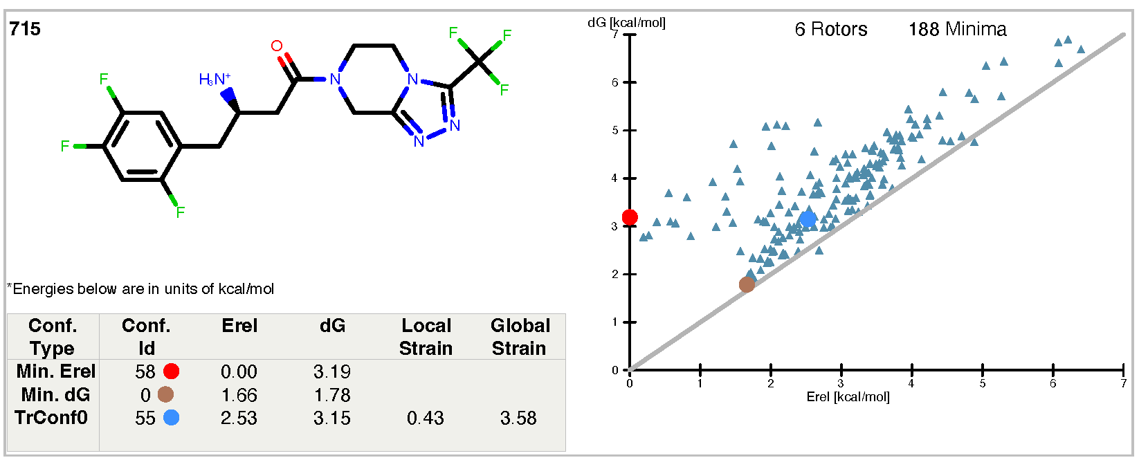
Results report from sitagliptin.mol2, using the “-track” flag

The results report in this case looks very similar to that of our first example except for the extra line added to the table and the corresponding extra dot (in blue) on the graph. The extra line in the table relates to the bioactive conformer specified in the input with the -track flag. “TrConf0” is an abbreviation for “Tracked Conformer 0”, that is, the first of the tracked conformers (in this case there was only one). The line beginning “TrConf0” gives information on the nearest unbound minimum to the tracked conformer, locating the unrestrained minimum from that conformer (in file sitagliptin.3D.pfn.tracked_free.oeb) and the corresponding relative energy (Erel) and conformer free energy (dG). The additional columns for this line give the local strain energy and the global strain energy associated with the tracked conformer.

These quantities are defined in the Freeform Theory section and depicted there in figure The components of Local and Global Strain Energies , but to briefly summarize: The local strain energy is the relative energy difference (internal energy + solvation energy) between the restrained energy minimum (the structure in file sitagliptin.3D.pfn.tracked_rstr.oeb) and the nearest unbound minimum (the structure in file sitagliptin.3D.pfn.tracked_free.oeb). Conceptually it corresponds to the energy required to distort the nearest unbound minimum to fit into the active site. The global strain energy is the sum of the local strain energy and the conformer free energy of the nearest unbound minimum.

Example 3

The third example is like the second except that PB single-point solvation energies are requested with the -solvent PB option. This is a higher level of continuum solvation theory compared to Sheffield solvation and so the solvation energies are expected to be more accurate. Sheffield solvation is still used in finding the minima for the unbound ensemble because it is fast and has the necessary analytic second derivatives. The command is:

prompt> freeform -calc conf -solvent PB -track sitagliptin.mol2 \
-in sitagliptin.mol2 -prefix sitagliptin.3D.pb.pfn

This produces eight output files analogous to those above for Example 2.

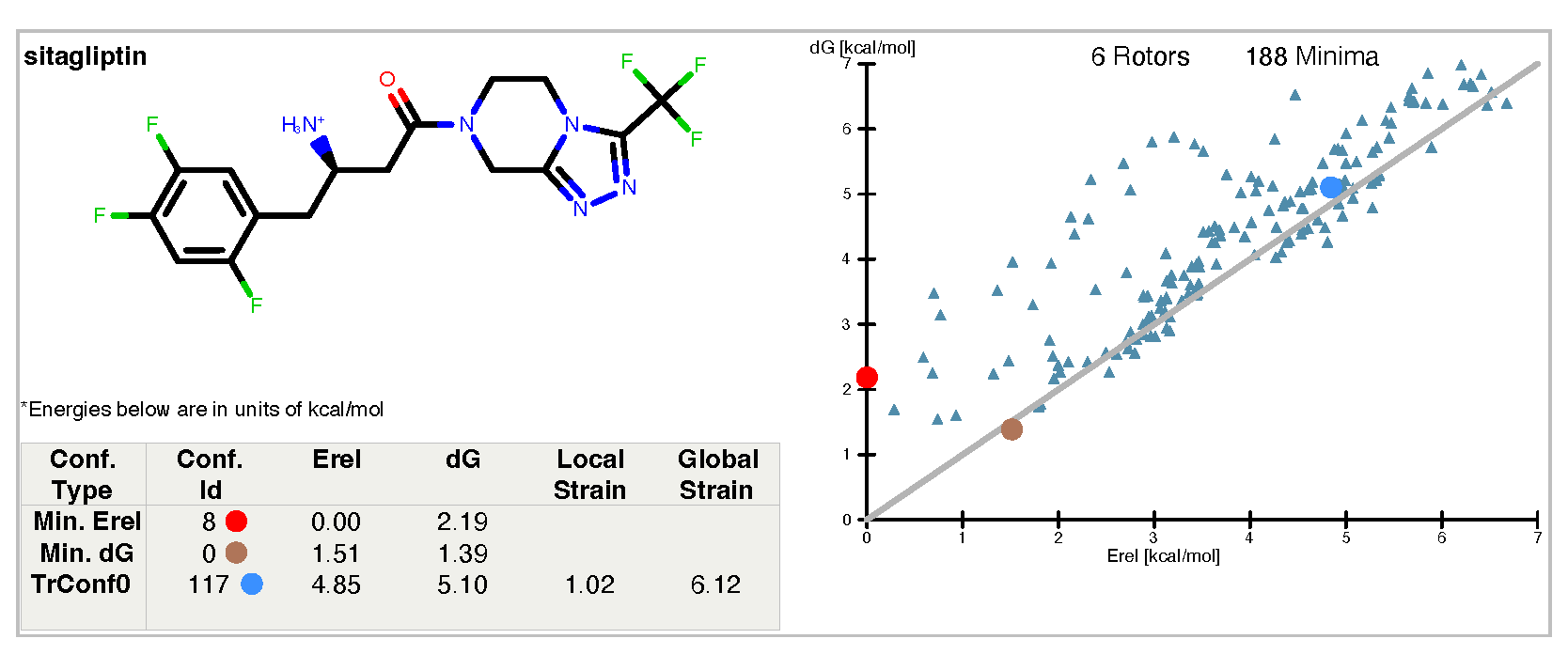
Results report from sitagliptin.mol2, using “-solvent PB”

Note that the energies and the graph differs markedly from that of Example 2. The partial charges, the number of unique minima, and the minima themselves are in both Example 2 and Example 3 found using the Sheffield solvation. The difference is the solvation energy for each conformer: in Example 2, the Sheffield solvation energy is used whereas in this example the Sheffield solvation energy has been replaced with a PB single-point solvation energy evaluated at the coordinates of the Sheffield-based minimum. The impact of changing to a PB energy is more pronounced with charged ligands.

Example 4

In the fourth and final example for freeform -calc conf, the same input file is used as in the second example, but now we would like to use the input charges in that file for the solvation energies. Note that in addition to specifying -solvcharges input we also need put -ionic input because the default behavior of potentially changing the ionic state for pH 7.4 cannot be allowed with input charges. The command is thus:

prompt> freeform -calc conf -solvcharges input -ionic input -track sitagliptin.mol2 \
-in sitagliptin.mol2 -prefix sitagliptin.3D.inp.pfn

The results report is in file sitagliptin.3D.inp.pfn.pdf and looks like:

Results report using “-solvcharges input``

Given that the only the atomic partial charges differ between this example and Example 2, we see significant changes in all the energies, yielding quite a different profile for the conformational ensemble. This includes changes to the conformer free energy and Global Strain Energy values for the nearest unbound minimum to TrConf0. These differences reflect the impact of using different charge models, especially on charged ligands; we recommend the default AM1BCC ELF10 charges.

Solvation free energies

Example 5

In order to estimate solvation free energy the user must use the option -calc followed by value solv. The default charge state of the input compound corresponds to pH = 7.4 (see option -ionic), so the following run:

prompt> freeform -calc solv -prefix januvia_ph74 januvia.smi

will estimate januvia solvation free energy at physiological pH. The graphical output file for this run is displayed in Figure: Solvation of januvia at physiological pH. On the left the result of the solvation free energy calculation is shown, including a depiction of the group-wise decompositions of the solvation free energy. It suggests that, as expected, the cationic \(NH_3\) group is responsible for almost all of the strongly negative solvation free energy of this molecule (-53.6 kcal/mol), while the trifluorophenyl fragment is the most hydrophobic part of this drug, adding to the solvation free energy (2.4 kcal/mol). To the right, the calculated XlogP partition coefficient is given together with its fragment decomposition into group contributions. Note that the calculated XlogP partition coefficient is always done relative to the uncharged molecule irrespective of its ionic state in water at any pH.

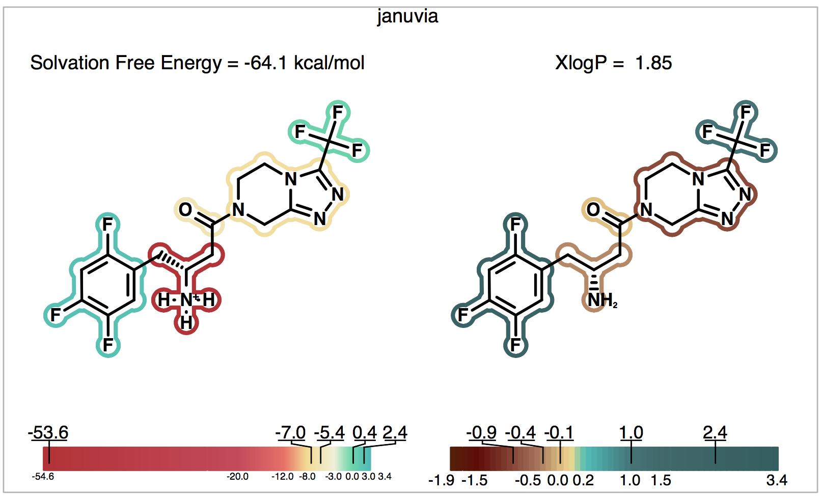
Solvation of januvia at physiological pH

Example 6

In the next example, the solvation free energy of januvia in its uncharged form is performed with:

prompt> freeform -calc solv -ionic uncharged -prefix januvia_neu januvia.smi

The output is shown in Figure: Solvation of the neutral form of januvia Note that changing the ionic state of the ligand only affects the solvation free energy on the left-hand side; the calculated XlogP partition coefficient is always done relative to the uncharged molecule so it is unchanged from the previous example. Now since the solvation free energy is also on the uncharged form, in this example (unlike the last) the solvation free energy and XlogP calculation correspond to the same (uncharged) form of Januvia.

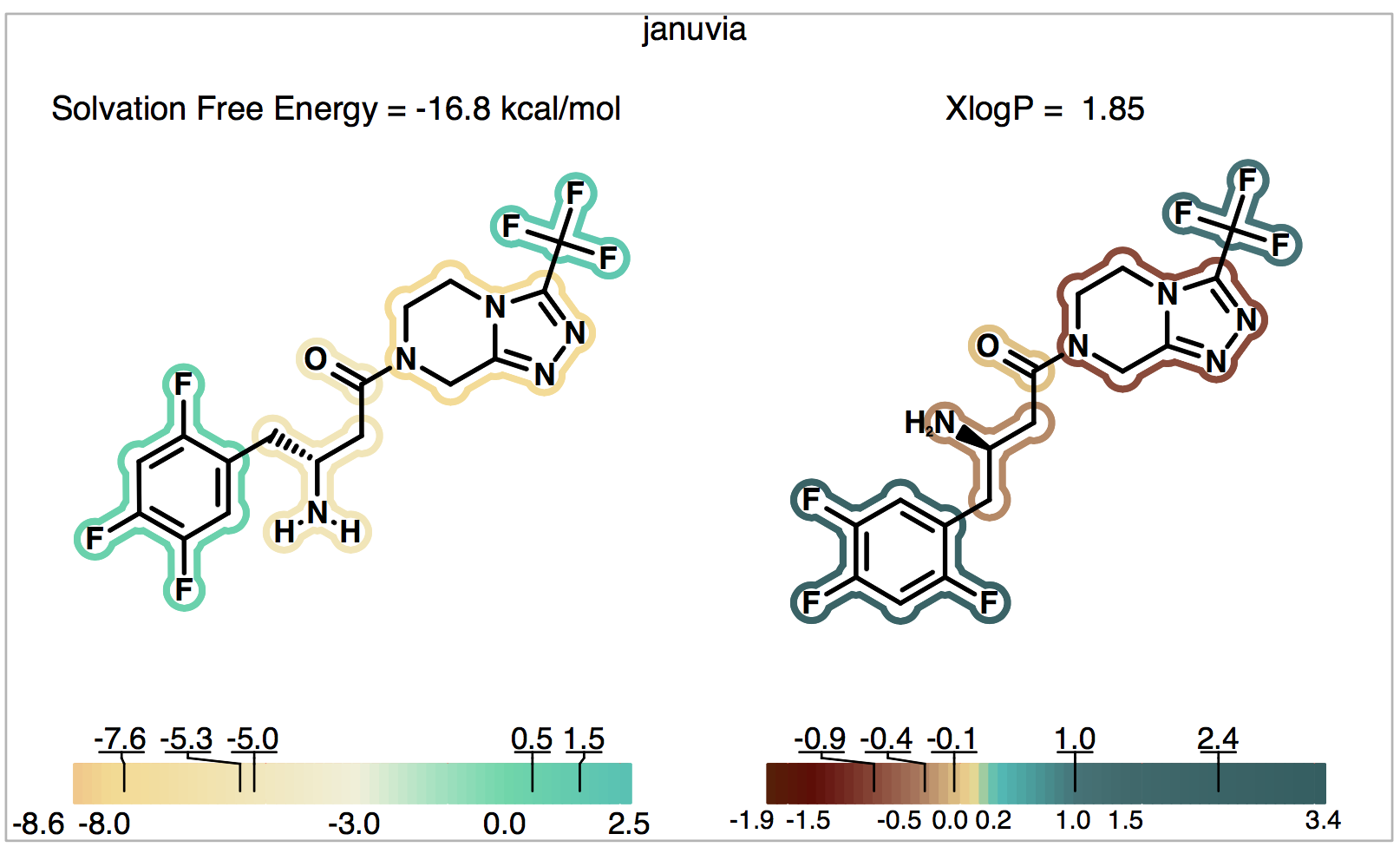
Solvation of the neutral form of januvia