Freeform Theory
freeform has two distinct functions:
“freeform -calc conf…”: Evaluation of the conformer free energy in solution, meaning the free energy required to select a particular conformer out of the whole conformational ensemble in solution.
“freeform -calc solv…”: Fast estimation of the small molecule solvation free energy and the XlogP calculated partition coefficient (with graphical representation of fragment-based contributions to these physical quantities).
Conformer Free Energies
Calculating the Partition Function
The method is based upon combining ligand conformational search, energy minimization, and entropy estimation in the workflow shown in Figure 1 below.
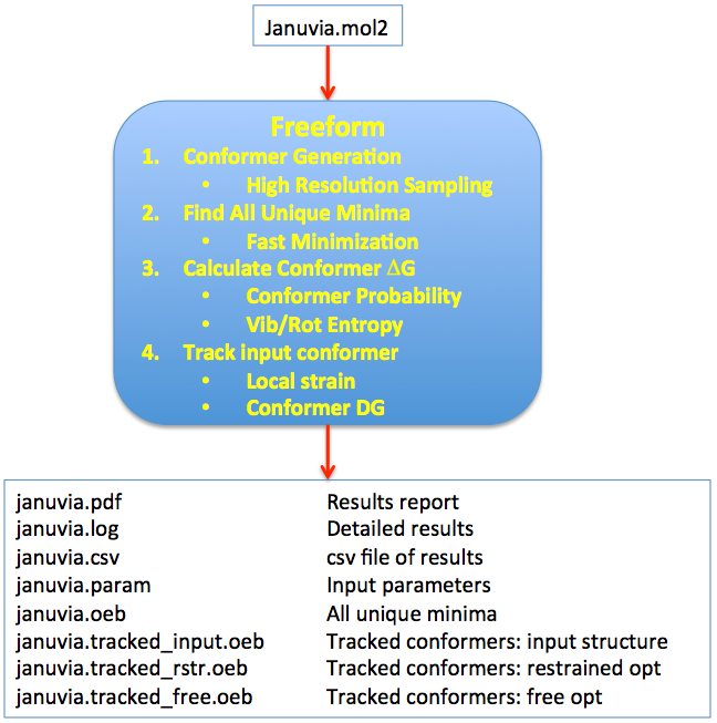
Figure 1. Stages and workflow in the conformer free energy calculation.
The conformational search is done at a very high resolution using the conformation generator OMEGA [Hawkins-2010]. The energy minimization uses Halgren’s MMFF94s force field [Halgren-VI-1999] and consists of several stages, all aimed at arriving at the most thorough sampling of the accessible conformational space of the ligand. Duplicate conformers are removed from the final minimized set, leaving an ensemble of \(n_c\) unique conformers, referred to below as the Ensemble of Unbound Minima, which we use to create an approximation to the partition function of the unbound ligand. This is illustrated conceptually in Figure 2.
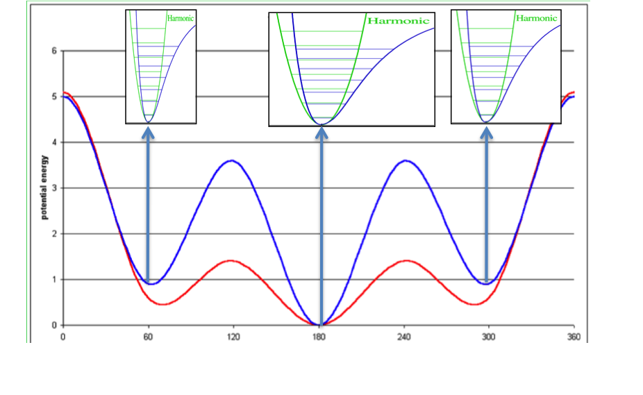
Figure 2. Concept of ligand entropy as a sum-over-states of conformer entropies.
To the molecule’s gas phase potential based on the MMFF94 force field (shown by the red line), Sheffield solvation energies are added to give a solvation-corrected potential (shown by the blue line) for which the minima are identified. The analytic second derivative of each minimum is then used to calculate the entropy contribution of each energy well according to Wlodek and coworkers [Wlodek-2010]. An energy minimum with a wider than average energy well will have a higher entropy, which will decrease the conformer free energy to select that conformer, while the converse will be true for a narrower than average energy well.
With this, the contribution \(Q_i\) of each energy minimum to the overall partition function \(Q\) can be calculated as
Here \(\epsilon_i\) is the relative internal energy (including solvation and zero-point energies) of the conformer relative to the global minimum conformation. \(q_t\), \(q_ir\), and \(q_iv\) are the translational, rotational, and vibrational partition functions, respectively, describing the entropic contributions from that conformation. \(n_c\) is the number of unique conformations in the ensemble. More details on these terms are given in the SZYBKI theory section. In practice, we do not compute the translational partition function \(q_t\) because it is constant for all conformers, so it cancels out of the conformer free energies.
Computing the Conformer Free Energies
Based upon this approximation of the partition function, we calculate conformer free energies: the free energy required to select a particular conformation from the unbound ensemble of all conformers equilibrating in aqueous solution. Strictly speaking, this is a Helmholtz free energy, not a Gibb’s free energy, because we are neglecting the differential PV (pressure*volume) contribution between conformers, but this should be negligible. Based on the above conformer and ensemble partition functions, the conformer free energy for any conformer is calculated straightforwardly as:
In addition to the graphic output file, which shows a plot of the calculated free energies of conformations versus their relative internal and solvation energies, energetic and thermodynamic results are stored in the log and CSV files.
Tracking Conformers
Often we are interested in one or more particular conformers, such as a
known or hypothetical bound conformer of a ligand (the “bioactive” conformer),
or perhaps a number of top-scoring poses from a docking run. One of Freeform’s
main purposes is to estimate the free energy cost of selecting such conformers
out of the unbound ensemble, a quantity we will refer to as the Global Strain Energy.
Freeform tracks these conformers using the freeform -track flag,
followed by the filename containing the input conformers for which ligand
strain energies are desired. Note that this is distinct from the input file
specified with the -in flag, which specifies the molecule from which
to construct the unbound ensemble. All conformers in the file specified after
the freeform -track flag will be tracked by freeform, and the user will
get a direct readout of the energy
required to select that particular conformation out of the aqueous ensemble.
Figure 3 shows how the various components of Local and Global Strain Energies are calculated.
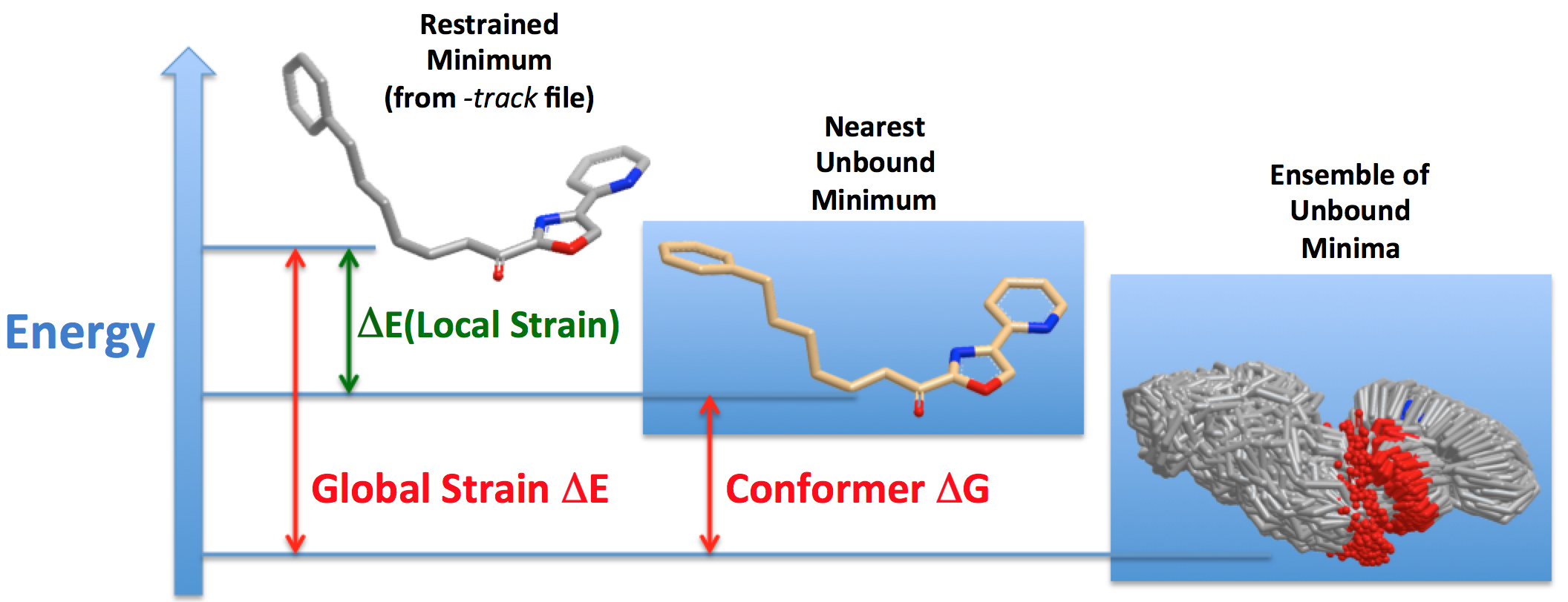
Figure 3. The components of Local and Global Strain Energies.
A key issue is that the input 3D coordinates of the tracked conformer may be of artificially high energy, usually due to small deviations of bond lengths and bond angles from the force field’s optimum values; this is often true particularly of ligands from X-ray structures. For this reason, the input structure is cleaned up with a restrained optimization using strong harmonic restraints to the input coordinates. The strong restraints retain the shape of the ligand (usually to within 0.2 Å RMSD) but resolve the artificially high energy. The energy of this restrained minimum structure is used in calculating the Local Strain Energy as shown in Figure 3 above.
Since conformer free energies must be calculated from energy minima in order to characterize the entropy, an unconstrained minimization is now required to find the Nearest Unbound Minimum to the input structure. This minimization allows the torsions in the input structure to relax away from where they may have been distorted from the nearby local minimum in order to fit into the active site. Freeform keeps track of this “distortion” strain energy as Local Strain Energy. From this point, Freeform simply includes the Nearest Unbound Minimum as just another energy minimum in the aqueous ensemble and calculates its conformer free energy, which is specifically reported in the PDF and log output (see examples). Thus, within Freeform, the Global Strain Energy for the input 3D structure would be considered to consist of a) the Local Strain Energy required to distort the Nearest Unbound Minimum, so the ligand can adopt the shape of the input tracked conformer, and b) the conformer free energy required to select the Nearest Unbound Minimum (i.e., the closest local minimum to the input structure) from the entire Ensemble of Unbound Minima.
Solvation Energy Estimation
How It Is Calculated
The term “solvation energy” is defined here as the standard free energy of transferring a compound from the gaseous phase into dilute aqueous solution, \(\Delta G_{solv}^{0}\).
Solvation energy is a crucial component of the solubility energetics and is directly related to hydrophilicity/hydrophobicity of a compound; therefore one can expect it is correlated with another measure of hydrophobicity, logP, as illustrated in Figure 4 below. Such a correlation, particularly when a functional group’s contribution is considered, might not exist. Freeform shows the graphical group contributions to solvation free energy and XlogP.
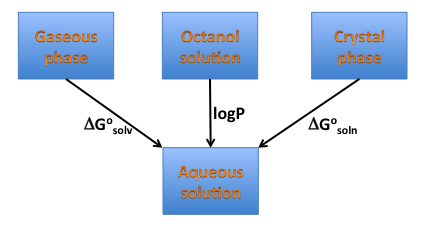
Figure 4. Solvation, solubility, and hydrophobicity.
The method is based on the continuum solvent model in which a Poisson–Boltzmann (PB) solver ZAP [Grant-2001] is used. The calculation is performed on the lowest energy gas-phase conformation found with the MMFF94 force field from the optimized set of conformations generated by the conformation generator OMEGA [Hawkins-2010]. A set of atomic radii ZAP9 and AM1BCC partial charges as described by Nicholls [Nicholls-2010] is applied for all PB calculations. Atomic and group contributions to the free energy of solvation for the input compound are calculated from atomic electrostatic potentials and atomic area terms representing the hydrophobic part of solvation. Assuming that a functional group has \(n\) atoms, its calculated solvation free energy \(\Delta G_s\) is
where \(V_{i,s}\) and \(V_{i,v}\) are calculated electrostatic potentials on atom \(i\) in solution and in vacuum, respectively, \(q_i\) is atom partial charge, and \(S_i\) is atomic contribution to hydrophobic part of solvation evaluated from a simple surface area model assuming 6.3 cal/(mol Å\(\AA\)) as a value for the microscopic surface tension coefficient. Graphical representation of group (or atomic) contributions to the free energy of solvation is performed with the OpenEye tools OEDepict TK and Grapheme™ TK.
Counterintuitive group contributions to solvation energies
Solvation free energy for molecular ions might not be trivial to interpret because of very strong intrinsic electrostatic interactions. One can most easily begin to understand these effects by considering zwitterions. A common zwitterion will contain both a group with a positive formal charge and a group with a negative formal charge. It is well known that zwitterions, though still having high solvation energies, have significantly smaller solvation energies than compounds with two formal charges of the same sign. In fact, zwitterion solvation energies are typically smaller than the solvation energy of the analog molecule with a single charge. For instance, as the examples in Figure 5 show, the solvation energy of zwitterionic phenylalanine is -35.4 kcal/mol, while the solvation energy of the formamide analog and the methyl ester analog are -74.9 and -64.6 kcal/mol, respectively.
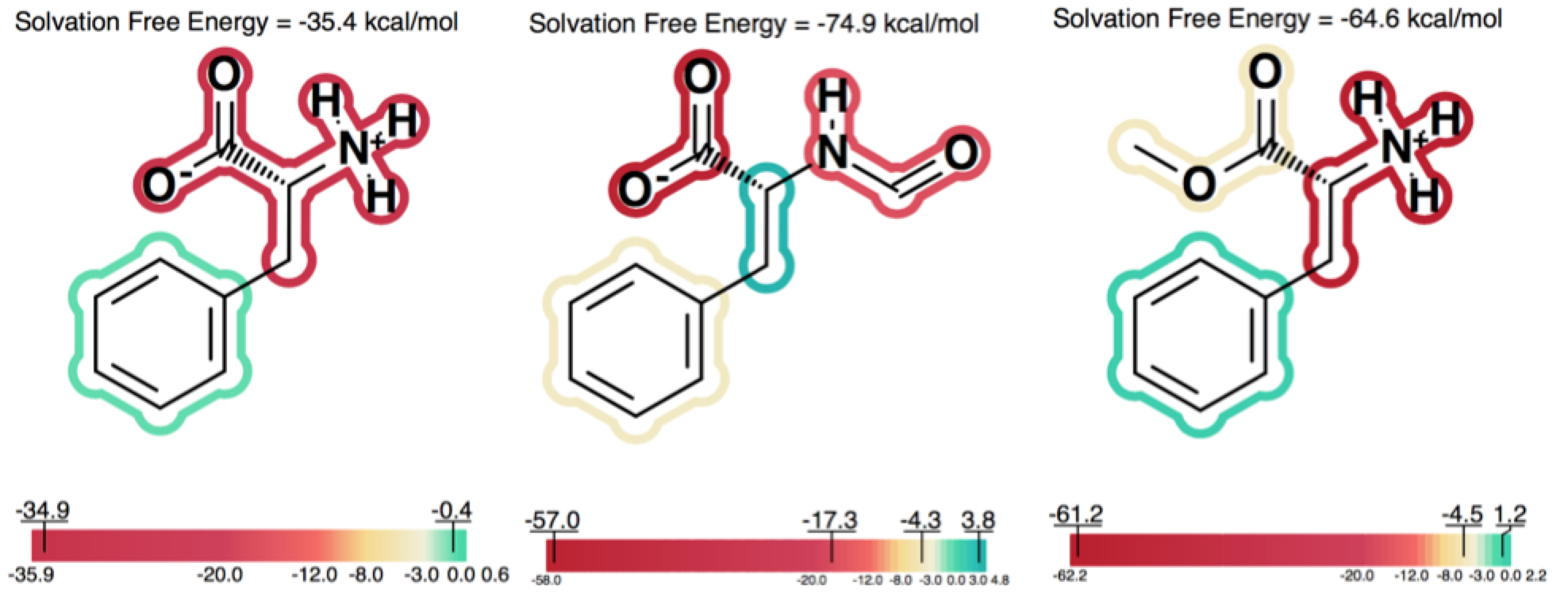
Figure 5. Solvation energy of zwitterionic phenylalanine and two singly charged analogs.
One can consider, then, that adding a charge of the opposite sign of the current molecular ion contributes a positive 30 to 40 kcal/mol to the solvation energy. A similar situation, perhaps even more dramatic, occurs in the case of intramolecular salt bridges, where positively and negatively charged groups are positioned in a very short distance. That kind of interaction does not only exist in macromolecules: NMR and hydrogen exchange rate experiments have also confirmed the presence of salt bridges between arginine or lysine and aspartate or glutamate side chains in short peptides ([Mayne-1998]; [Otter-1989]). Making positive contributions to the solvation energy is generally considered a hydrophobic effect, yet here the contribution is made by a charged species, which is somewhat counterintuitive at first. Nevertheless, in this context, one can understand how, under the right conditions, a normally hydrophilic functional group can make a significant positive contribution to the solvation energy. The more confusing circumstance is when, rather than a simple zwitterion, we see a similar effect in a molecule with either multiple charges of one type (either positive or negative) and a single charge of the opposite sign. Consider a molecule with 2 negative ions, one positive ion and a total charge of -1, like the one shown in Figure 6.
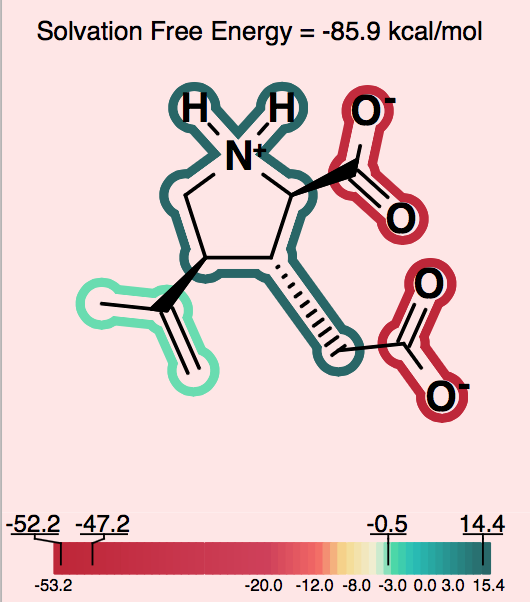
Figure 6. Counterintuitive group contributions to solvation.
In this case, the positive ion will change the formal charge from -2 to -1. This will make the total solvation energy significantly less negative (a positive contribution to the solvation energy). The positive ionic functional group in this case will have a large positive solvation energy. While a charged group is indeed not hydrophobic, in this instance, one can understand that it makes the solvation energy less negative in a manner similar to the way a hydrophobic group might, but to a larger degree. In more subtle cases, one can observe a similar though less dramatic hydrophobicity in a molecule with a single charge, either positive or negative, and another fragment that makes a large neutralizing contribution to the partial charge of the molecule.
In order to alert the user, species which contain strong intramolecular electrostatic interactions of the nature described above are depicted on a light pink background. This should act as a reminder to users to consider the net charge of the molecule in interpreting the relative contribution of each fragment to the solvation energy.