3D Display
The 3D display is the primary visualization interface available to the user (although it is not the only one, there is also a spreadsheet view and 2D views). The purpose of the 3D display is to allow the user to view and interact with molecules, grids, and surfaces.
User Interaction
The primary interface mechanism to the 3D display is the mouse which is discussed in detail below. However, the large number of potential operations that can be performed in the 3D display necessitate an additional mechanism of interaction besides the simple use of mouse buttons and popup menus. For this reason a separate peripheral window is provided to access these operations. This window is called the Style Control and is discussed below.
Mouse
As described above, the mouse is considered to be the primary interface mechanism to the 3D display. The details of how to use the mouse to interact with the 3D display are listed here. A three (or two) button mouse is recommended for use; however, support for a single button mouse is available on macOS. Holding down the Ctrl key while clicking or pressing the mouse button will emulate using the Right mouse button on a three button mouse.
For users not comfortable or familiar with the mouse interactions described below, VIDA can be made to emulate the mouse behavior of many other applications including: Coot, Insight, Maestro, MOE, O, Quanta, PyMol, RasMol, and SYBYL. The desired mouse map can be set in the application preferences in the 3D Display section (Figure: Mouse Map Preferences). Please note that not all the functionality described below is available in the emulated mouse modes, nor is all of the functionality of the emulated applications available in VIDA.
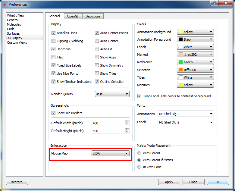
Mouse Map Preferences
Selection
Objects in the display can be selected by clicking on them using the Left mouse button. The selection is cleared between button clicks (or by clicking in the background) unless the Shift or Ctrl key is also held down when clicking. If a single atom on a surface has been selected, holding down the Shift key and selecting a second atom will select the shortest path of vertices between the two selected end points.
Double-clicking using the Left mouse button expands the current selection to the next logical grouping. For instance, double-clicking on a selected atom in a protein will expand the selection to include all of the atoms in the same residue as the original selected atom. Double-clicking on the selected set again will expand the selection to include either the entire chain if there are multiple chains, otherwise it will include the entire molecule.
Selection can also be performed using a lasso style selection method by holding down the Right mouse button and moving the mouse in the window to define a selection rectangle (a dotted rectangle will be displayed on the screen as you do this). Releasing the Right mouse button will select all of the atoms and bonds inside of the rectangle. The previous selection will be cleared unless the Shift or Ctrl key is also held down while moving the mouse. Lasso style selection of surfaces and grids is not currently supported.
Additional methods of selection are available in the Select Menu pane of the Style Control and the Select Menu.
Rotation
The scene can be rotated in three dimensions by holding down the Left mouse button and moving the mouse in the window. These movements will emulate rotation using a trackball.
The scene can also be rotated around just the Z axis by holding down the Alt key and the Left mouse button simultaneously.
Translation
Using the mouse, the scene can be translated in the XY plane by holding down the Shift key and the Left mouse button simultaneously. Translation along the Z axis can be performed by holding down the Alt key, Shift key, and the Left mouse button simultaneously. The scene can also be translated along the Z axis by holding down the Alt key while using the mouse wheel.
Using the keyboard, the scene can be translated horizontally in the display by pressing either the A key or D key which translate to the left and to the right respectively.
Scale/Zoom
The scene can be scaled (or zoomed) by holding down the Middle mouse button by itself, the Left and Right mouse buttons together, or by using the mouse wheel. Any of these three modes will scale the scene. Multiple modes are provided for convenience and to accommodate the many varied mouse configurations in existence.
The scene can also be scaled using the W and S keys on the keyboard.
Text Scale
The scale of the text displayed in the scene can be controlled by using the mouse wheel while holding down the Ctrl key.
Clipping
The position of the near and far clipping (or slabbing) planes can be controlled using the mouse wheel while holding down both the Ctrl and Shift keys. Both planes are moved simultaneously and mirror each other’s position. It is important to note that slabbing must already be enabled for these operations to actually be performed.
The clipping planes can be adjusted independently by holding down the Alt key with one of the Ctrl or Shift keys corresponding to the far and near clipping planes respectively.
Contour Level
The contour level of the grids in the default scope can be adjusted using the mouse wheel while simultaneously holding down the Shift key. Each incremental turn on the mouse wheel corresponds to an increase or decrease in the contour level by 0.1.
Label
Informative labels can be displayed about atoms and bonds (as well as surfaces and grid contours) underlying the current mouse position if the Ctrl key is pressed while moving the mouse (no mouse button need be depressed) on most platforms. On the Mac, this behavior is obtained by holding down the Alt key instead of the Ctrl key.
Additional methods of labeling atoms and bonds are available in the Style pane of the Style Control .
Style Control
The Style Control is a separate peripheral window which is provided to enable additional interactions with the 3D display. The Style Control is a vertical window consisting of many individual panes. Each pane provides its own set of functionality. The display of the individual panes can be toggled by clicking on the title bar of the pane of interest. In addition, individual panes can be “torn off” to act as top-level windows by clicking on the “+” icon in the top right of the title bar. When the pane is torn off the “+” icon becomes a “-” icon which when clicked hides the “torn off” window. The specific details of the individual panes are listed below.
Color
VIDA provides a wide array of coloring schemes as can be seen in the color pane (see Figure: Color Pane). The first button (with the color wheel icon) prompts the user to select a specific color which will be applied to all of the objects in the current scope. The second button (with the molecule overlaid on a color wheel) prompts the user to select a specific color that will be applied to all molecules in the current scope. In addition, this button contains a drop down menu of molecule specific coloring schemes which can be applied. Detailed information about the individual color schemes can be found in Molecule Color. The third button (with the surface overlaid on a color wheel) prompts the user to select a specific color that will be applied to all surfaces in the current scope. In addition, this button contains a drop down menu of surface specific coloring schemes which can also be applied. Detailed information about the individual color schemes can be found in Surface Color. The fourth button (with the grid overlaid on a color wheel) prompts the user to select a color that will be applied to all grid contours in the current scope. The fifth button (with the “U” icon overlaid on a color wheel) assigns a unique color to every object in the current scope. The last button restores the original color of all the objects in the current scope. More details about the specific coloring schemes can be found below.
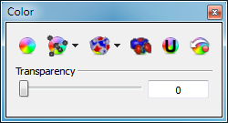
Color Pane
Beneath the buttons is a slider which can be used to adjust the transparency of surfaces (see Table: Surface Transparency) and grid contours. The slider values range from 0 (completely opaque) to 100 (completely transparent). The specified transparency value is applied to all surfaces and grid contours in the current scope. However, if a part of a surface is selected, the transparency will only be applied to the selected region as can be seen in the second figure in Table: Surface Transparency.
|
|
Transparent surface |
Partially transparent surface |
Selection
The simplest mechanism to perform a selection is to click on the object of interest in the 3D display using the mouse. However, a number of additional selection mechanisms are available in the selection pane as can be seen in Figure: Selection Pane.
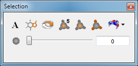
Selection Pane
In the top row of the selection pane, there are seven individual buttons. The first button with the “A” icon selects all of the currently visible molecules. The second button with the partially selected molecule icon performs a selection based on a substructure query. Clicking on this button will launch a query dialog which allows the user to specify a substructure query. The substructure can be entered as a SMARTS pattern, selected from a large number of predefined patterns, or can be specified using a common or IUPAC name which will be converted to a structure using OpenEye’s Lexichem toolkit. All atoms in the current scope matching the specified pattern will be selected. If the current scope is set to All and more than 50 molecules match the pattern, the user will be prompted as to whether to Mark the matching structures instead of selecting them, as being selected would make them visible.
The third button inverts the current selection, unselecting everything that was selected and selecting everything that is currently visible but was not previously selected. The fourth button selects everything within a defined radius of the current selected set (the default is 5 Angstroms). The fifth button selects everything within a user specified radius of the current selected set. This radius is specified by the slider in the bottom row of the pane. The sixth button selects everything outside of the same user specified radius of the current selected set. It is important to note that these distance based selection mechanisms expand their selected sets to include entire residues in the event that only a portion of a residue is included within the radius.
The last button contains a drop down menu which has different options based on the current selection. If a molecule is selected it contains the following options: “Hide Outside”, “Hide Inside”, and “Restore”. Selecting one of these options will hide all of the atoms and bonds outside the current slider specified radius, hide all of the atoms and bonds inside the current slider specified radius, or unhide any previously hidden atoms and bonds respectively. If a surface is the options are: “Crop Outside”, “Crop Inside”, and “Restore”. Selecting one of these options will crop away the unselected portion of the surface, crop away the selected portion of the surface, or restore the surface to its original state respectively. Examples of cropped surfaces can be seen in Table: Surface Cropping.
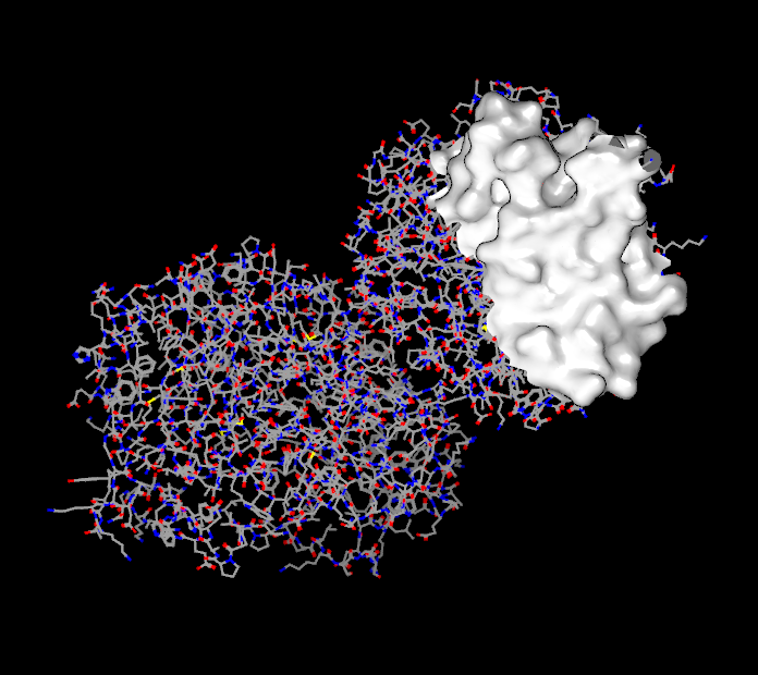
|
|
Unselected region removed |
Selected region removed |
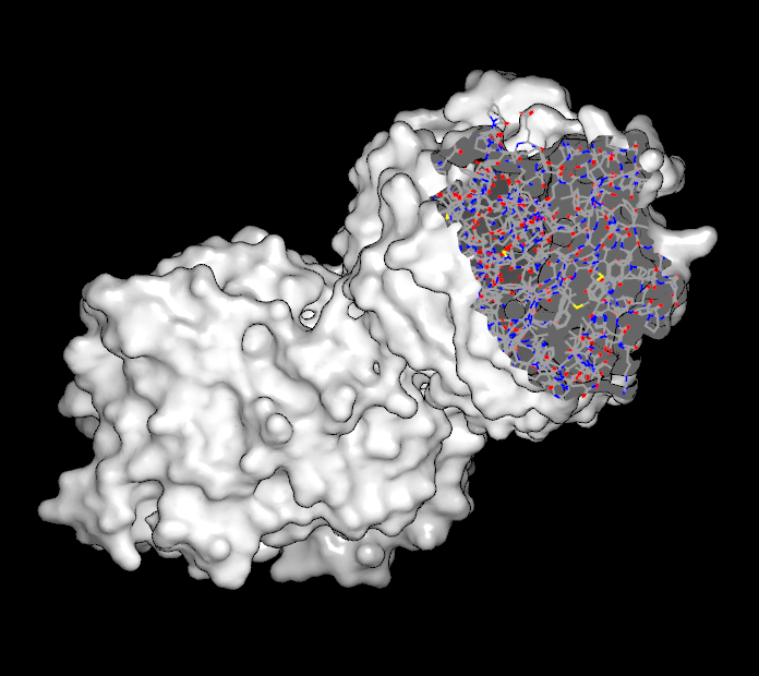
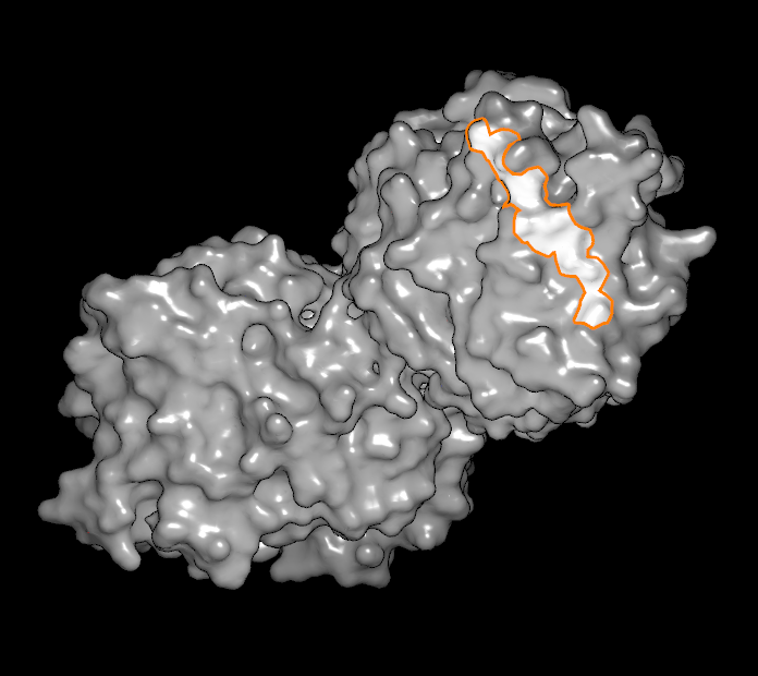
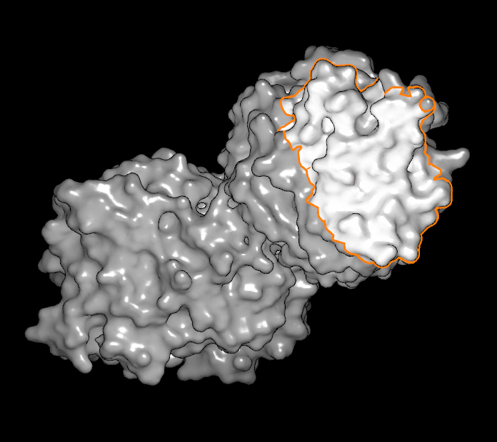
In the bottom row, there is one button adjacent to a slider and a numeric display. The button is a toggle that controls whether or not unselected atoms and bonds are shown based on their distance to the selected set. The cutoff distance is controlled by the adjacent slider (and the actual value in Angstroms can be seen in the numeric display). This state of this button is ignored when a surface is selected. When a vertex (or a line of vertices) is selected, the slider can be used to flood out from the original selected set to include many more adjacent vertices. The different types of surface selections can be seen in Table: Surface Scribing.
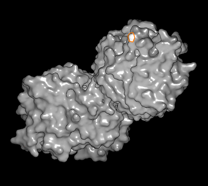
|
|
|
Single atom selected |
Line of atoms selected |
Region of surface selected |
Style
The style pane of the Style Control is divided into two distinct areas as can be seen in Figure: Style Pane. The area above the dividing line contains a row of four buttons which control the display style of the various different types of objects that can be visualized in VIDA. The area beneath the dividing line is a collection of buttons whose functionality is specific to just molecules.
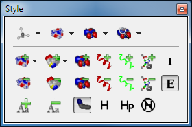
Style Pane
In the top area, the first button (with the molecule icon) contains a drop down menu of the available molecule display styles: ball and stick, CPK, stars, stick, wireframe, and hidden. Selecting one of these options will change the display style of all the atoms and bonds in the current scope.
The second button (with the surface icon) contains a drop down menu of the available surface display styles: solid, mesh, and points. Selecting one of these options will change the display style of all the surfaces in the current scope.
The third button (with the grid icon) contains a drop down menu of the available grid display styles: solid, line, and cloud. Selecting one of these options will change the display style of all the grid contours in the current scope.
The fourth button contains a drop down menu of the supported grid types in VIDA: Electrostatic, ET, FRED, Generic, Difference Map, and Regular Map. Selecting one of these options will change the grid type of all the grids in the current scope. A grid’s type determines how it is visualized in VIDA including the default number of contours (and their levels) and the display style as well as the color of those contours.
In the bottom area, there are three individual rows of buttons. In the first row, the first three buttons turn on the display of molecular surfaces, accessible surfaces, and electrostatic grids, respectively. Surfaces are created over the selected atoms, or over the currently scoped molecule if no atoms are selected. The two surface buttons have pulldown menus to allow either toggling the visibility of a surface or regeneration of the surface. Regeneration may be used to surface a new part of a molecule if the selection has changed. Surfaces and grids generated with these buttons are considered display properties of their associated molecules and therefore are not displayed in the List Window. Independent (non-property) versions of these can be created from the relevant options in a right-click menu. The next two buttons turn on the display of protein ribbons and c-alpha traces respectively. The next button turns on the display of hydrogen bonds by making all of the molecules in the current scope to be hydrogen bond targets. Being a hydrogen bond target means that when it is visible, it displays any hydrogen bonds made between it and any of the other molecules that are also visible. The last button in the row toggles whether or not internal (intramolecular) hydrogen bonds are shown.
In the second row, the first three buttons turn off the display of molecular surface, accessible surfaces, and electrostatic grids, respectively. The next two buttons turn off the display of protein ribbons and c-alpha traces. The next button makes all of the molecules in the current scope no longer hydrogen bond targets. The last button in the row toggles whether or not external (intermolecular) hydrogen bonds are shown.
In the last row, the first button allows the user to specify and turn on atom and bond labels. The second button turns off all of the atom and bond labels in the current scope. The third button toggles the display of non-bonded atoms in the scene. The remaining three buttons control the hydrogen style for the molecules in the current scope. The first of the three turns all hydrogens on, the second buttons shows only polar hydrogens, and the last button hides all hydrogens.
Contours
|
|
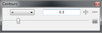
Normal view |
Advanced view |
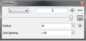
The contour pane of the Style Control is used to control the number and level of the individual grid contours as can be seen in Table: Contour Pane. When the current application scope is set to Focused there will be a pull down menu in the top left of the window containing a list of all the current grid contours. If the scope is not set to Focused, the scope will be displayed in place of the pull down menu to remind users that all operations in this window apply to more than just the Focused grid. Next to this area is a numeric display which displays the current contour level. Next to this display are two buttons, one with a “+” icon and one with a “-” icon. These two buttons allow for the creation and deletion of individual grid contours. Please note that these options are disabled for both Electrostatic and ET grids as they can have only two contours: positive and negative. Furthermore, the contour levels of the positive and negative contours are coupled together and so changing one will change the other (but with the opposite sign).
At the bottom of this window is a slider which allows for direct control over the contour level. To the right of the slider is an Advanced button (with the equalizer icon) which will expand the pane to show a number of advanced options (see Table: Contour Pane).
In the advanced section, there are two adjustable parameters (Radius and Grid Spacing) and one button. The parameters control how contours of Reentrant grids are displayed according to their symmetry. The Radius parameter specifies how far out from the center of the scene (in Angstroms) VIDA should look in the grid in order to generate of the isocontour. The Grid Spacing parameter specifies the spacing (in Angstroms) of the sub-grid used to generate the isocontours.
The single button (with the check icon) to the right of the Radius parameter converts the current grid contour into a fixed surface independent of the grid. This can be particularly useful when generating state files as a single surface can take up considerably less disk space than an entire grid.
Graphics
The graphics control pane in the Style Control provides an additional level of control over and interaction with the 3D display (see Figure: Graphics Pane). It is particularly useful for users without mouse wheels.
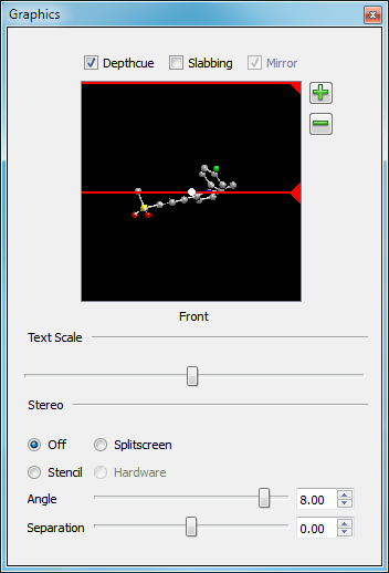
Graphics Pane
At the top of the graphics pane are three check boxes: “Depthcue”, “Slabbing”, and “Mirror”. The first two check boxes toggle the use of their associated properties respectively. The “Mirror” check box is only enabled when slabbing is on and controls whether the front and back slabbing planes move together (mirrored around the center of the scene) or independently.
Beneath these check boxes is an interactive control which allows the user easy control over both depthcueing and the clipping planes. Displayed in the control is a top-down view of the current scene in the 3D display. The front of the scene is at the bottom as indicated by the label.
When depthcueing is enabled, two red lines will appear in the control which indicate the start and the end points in the depthcueing calculation. These lines can be moved by clicking on the triangular tab at the right of the lines and dragging them to the desired location. The 3D display will update dynamically as these lines are moved.
When clipping (or slabbing) is enabled, two yellow lines will appear in the control which indicate the position of the near and far clipping planes. These can be moved by simply clicking on the triangular tab at the left of the lines and dragging them to the desired location. The 3D display will update dynamically as these lines are moved.
In the center of the control is a small white dot that corresponds to the center of scene that the camera is pointing at. The position of the center can be changed in the Z plane by dragging the dot in the vertical plane. The position of the center can be changed in the X plane by dragging the dot in the horizontal plane.
Beneath this control is a slider which controls the scale of the text drawn in the 3D display. The 3D display will update dynamically as the slider is adjusted.
Beneath the slider are four radio buttons which control the mode of stereoscopic visualization. The default behavior is “Off”. The “Stencil” option provides an additional mechanism for hardware stereo specific to the Zalman Trimon 3D LCD Monitor.
Custom Views
Each of the individual custom views available in VIDA can also provide their own individual panes which can be inserted into the Style Control to further enable task specific operations. These panes appear when a specific custom view is selected and disappear when the “X” icon is clicked or when another custom view is loaded. For more information on custom views refer to the Custom Views chapter.
Rendering
The images shown in the 3D display are rendered using OpenGL, therefore the quality and speed of the rendered scenes in the 3D display is dependent on the graphics card in the computer running the application. Computers with graphics cards that do not support OpenGL acceleration will still be able to display images, but the quality and speed with which the images are displayed may be markedly reduced. To help alleviate situations like this, multiple “levels of detail” are supported ranging from “Fastest” to “Best” which adjust the quality of the rendered scenes accordingly. For most computers, “Best” level of detail should be appropriate. “Presentation” quality rendering is optimized for creating images with a white background, such as might be used in slide presentations and printed documents.
In addition to the “level of detail”, the scene can be further adjusted by modifying a few select OpenGL parameters such as the background color as well as the lighting and material models. All of these parameters can be adjusted in the application preferences.
Stereo
Multiple types of stereo visualization are supported in the 3D display. The “Stencil” option enables stereo visualization using the Zalman Trimon 3D LCD Monitor. This is the only LCD display on which stereo visualization is supported. This monitor has been tested on multiple operating systems and requires no specific graphics card.
Finally, split-screen stereo is also a viable option. Both cross-eyed and wall-eyed views are available and can be set in the preferences. Furthermore, the stereo angle and eye offset parameters can be adjusted in the preferences as well.
Viewpoint
When viewing objects in the 3D display, there is always a center to the scene
where the virtual “camera” is pointing. When the first molecule, grid, or
surface is loaded into the application, the center of that object becomes the
center of the scene where the camera is pointing. By default, the center does
not automatically change with changes to the scene. The center can be changed
explicitly from the main application toolbar, the right-click popup menu, or
using the following scripting commands: ViewerCenterSet or
ViewerCenterAndRadiusSet. Furthermore, the center can
also be translated using mouse interactions.
The center can be made to automatically change when browsing if the “Auto-Center” or “Auto-Fit” preferences are set to true (the default is false). The “Auto-Center” preference directs the window to always recenter the scene after any changes are made to that scene. The “Auto-Fit” preference directs the window to not only recenter the scene after any changes are made but to also ensure that everything in the scene is completely visible in the window. These preferences can be edited in the application preferences dialog.
Bookmarks
The 3D display is capable of capturing and storing named bookmarks of the currently displayed scene to enable viewing again at another time without having to setup the scene again by hand. Bookmarks are saved in state files and are particularly useful when trying to communicate multiple pieces of information to other users.
All bookmarks have names and are stored in order. Bookmarks can be created from the top-level Bookmark menu by selecting the “Add” option. The order of the bookmarks can be organized by selecting the “Organize” option in the same menu. The Bookmark menu also contains an “Animated” option which controls whether VIDA animates the transition between the current scene and the newly selected bookmark. A list of all the currently available bookmarks populate the rest of the menu. Bookmarks can also be created by clicking on the “Add Bookmark” button in the 3D display Style toolbar.
The 3D display also provides a bookmark display widget which displays a clickable list of all the available bookmarks directly in the 3D display.
Tiled Display
The default behavior of the 3D display is to display everything that is Visible in the same coordinate space; however, there are often occasions when it is desirable to view everything in their own space. This behavior can be obtained in “Tiled” mode, also called “Matrix” mode or “Multi-Pane” mode. “Tiled” mode can be toggled on or off from the main application toolbar.
When the 3D display is in “Tiled” mode every Visible and Focused object is displayed centered in its own individual pane. However, if desired each object can be shown relative to the same center if the “Auto-Center Panes” option in the 3D Display section of the application preferences is unchecked. It is important to note that when “Auto-Center Panes” is enabled it is not possible to recenter or translate using mouse interactions in any of the panes.
To indicate which object is Focused, the corresponding pane will contain a blue border just inside the regular pane border. If there are any Locked objects, each of them will be displayed in every pane in addition to the individual Visible and Focused objects.
Toolbars
The 3D display provides additional toolbar areas (aside from the main application toolbar) inside the 3D window. There are four possible toolbar locations: at the top of the window, at the bottom of the window, at the left edge of the window and at the right edge of the window.
By default, the 3D display provides a “Mouse” toolbar at the left edge of the display. In Edit mode, a “3D Right” toolbar on the right side of the display is populated with building tools. Two toolbars are empty and hidden by default, one at the bottom of the 3D Window (“3D Bottom”) and one at the top (“Style”). These can be shown and populated via the use of scripting commands.
Mouse Toolbar
The Mouse toolbar contains a single row of buttons along the left side of the 3D display which control the behavior of the mouse in the display. The first button is the default and puts the mouse into normal selection mode. The second button puts the mouse into information mode which will cause information about the object currently under the mouse to be displayed. The third button puts the mouse into centering mode which will cause the display to be centered on whatever the mouse clicks on. The fourth button puts the mouse into measuring mode. There is a drop down menu adjacent to this button which allows the user to select one of three measurement modes: Distance, Angle, and Torsion. The fifth button puts the mouse into labeling mode which will prompt the user for a custom label to apply to any object that is clicked.
Double-clicking in the background of the 3D display will restore the mouse function to the default selection mode.
This toolbar can be referenced in scripting commands using the name “Mouse”.
Bottom Toolbar
Although empty by default it contains a set of buttons (that change depending on what is active) collectively referred to as the “Object toolbar” although they are not technically a separate toolbar. It also contains the bookmark widget.
For each type (molecule, grid, surface) it can show two buttons which represent menus - one color & one style. If the active object is a molecule and it has surfaces and/or grids shown via the Style Control, it will show the button menus for those objects as well. These buttons are quick links to the options available in the Style Control window.
This toolbar can be referenced in scripting commands using the name “Bottom”.
Right Toolbar
This toolbar is displayed during 3D building, and contains tools for editing molecules. The first button is a tool for deleting atoms and bonds. The second button shows a benzene ring by default and attaches the fragment selected from a dropdown to either an atom or bond of the molecule in the main window. The third button provides a dropdown for selection of the active atom type. The fourth button provides a selection of bond types from a dropdown. The fifth button allows modification of format atomic charges. The sixth button allows stereochemistry to be set (R/S or E/Z) or inverted. The last tool on this toolbar minimizes the active molecule using the MMFF94 or MMFF94s forcefield.
Application Toolbar
In addition to providing its own toolbars, the 3D display is affected by a few of the buttons in the main application toolbar. The application toolbar contains the “Tiled” display toggle button (matrix icon), the main window screenshot button (camera icon), the centering button (four arrows pointing in), the fitting button (four arrows pointing out), the new molecule button, and the edit molecule button.
The “Tiled” display button toggles the display between single pane overlay mode and multiple pane tiled mode. The screenshot button captures an image of the current main window at a user specified resolution. The centering button centers the display on the currently selected set or whatever molecule(s) are in the current scope. The fit button centers the scene and adjusts the scale factor such that all Visible objects can be seen on the screen at the same time. The new molecule button prompts the user to specify a new molecule using the 2D molecule editor. The edit molecule button puts the application into editing mode for the currently active molecule.
Display Widgets
The 3D display provides a number of additional widgets which are drawn directly in 3D display as opposed to on the side or floating above it. These widgets include an annotation widget, a bookmark widget, a data display widget, and a depiction widget. See Figure: 3D Display Widgets.
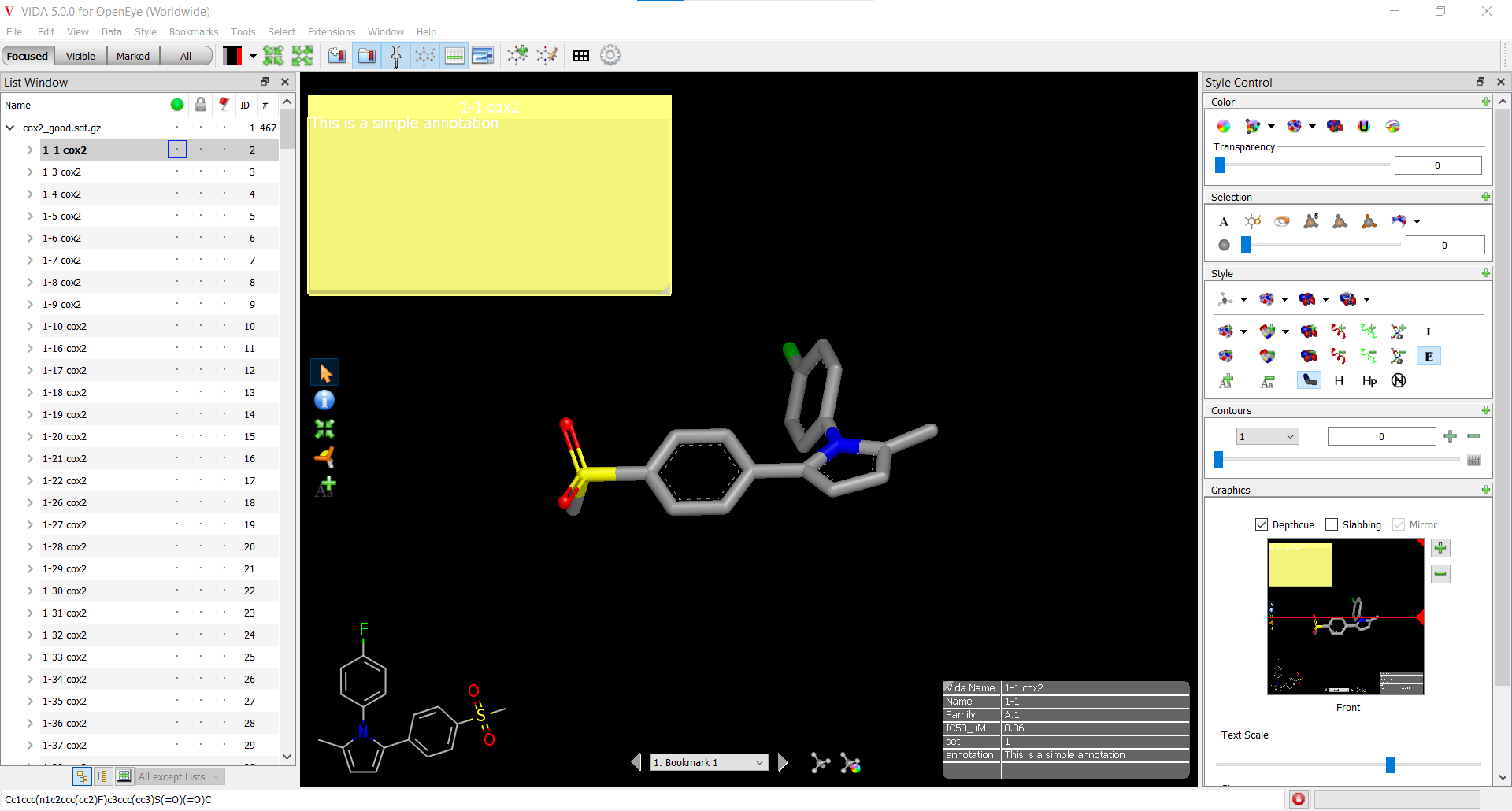
3D Display Widgets
Annotation
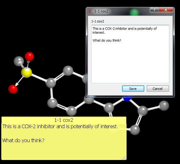
It is often desirable when viewing molecules to make notes or simple annotations about specific molecules. This can be done directly within the 3D display, where the annotation widget appears like a transparent Post-It(TM) (see Figure: Molecule Annotation). The color of the widget as well as the font used can be specified in the application preferences.
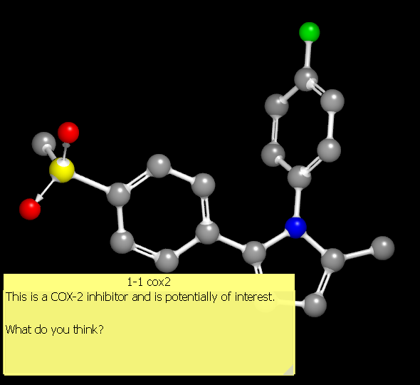
Molecule Annotation
The widget can be moved by clicking on the title bar and dragging it to the desired location. The widget can be resized by grabbing the small triangular tab in the lower right-hand corner of the widget and dragging until the desired size is achieved.
Clicking in the annotation widget will activate it for editing. Editing can be accomplished by directly typing once the widget has been clicked or by clicking on the “Edit” button in the title bar. Clicking on the “Edit” button will launch a more fully featured text editor which supports copy and paste operations (see Figure: Annotation Editing).
Annotation Editing
Annotations are also stored in the spreadsheet and can be edited there as well as in the 3D display. Annotations are saved as a SD tag when a molecule is written out (in either SD or OEB formats).
Bookmark
The bookmark widget is a simple widget drawn at the bottom of the 3D display (Figure: 3D Display Widgets) containing a clickable list of the currently available bookmarks. Clicking on any individual bookmark will load that bookmark and update the display accordingly.
Data Display
This widget provides a simple table which contains the spreadsheet data of the Focused object. The widget can be moved around the 3D display by clicking and dragging it to the desired location. It can also be resized by clicking in the tab in the upper left hand corner. Lastly, if the amount of data associated with the object is too large to be shown all at once, the widget does provide scrolling functionality.
Depiction Widget
The depiction widget draws a 2D depiction of the focused molecule directly into the 3D display. The depiction is drawn in the lower left hand corner of the display (or individual pane if in tiled mode). The depiction style is determined based on the application 2D depiction preferences. The size and other drawing parameters (e.g. anti-aliasing) of the depiction are also specified in the application preferences.
The depiction widget is mouse-aware making it possible to perform selections in this region.
Molecular Visualization
This section describes the very powerful, versatile, and interactive molecular visualization capabilities of the 3D display. The interactive control of molecular visualization is typically performed using the Style Control or through scripting commands.
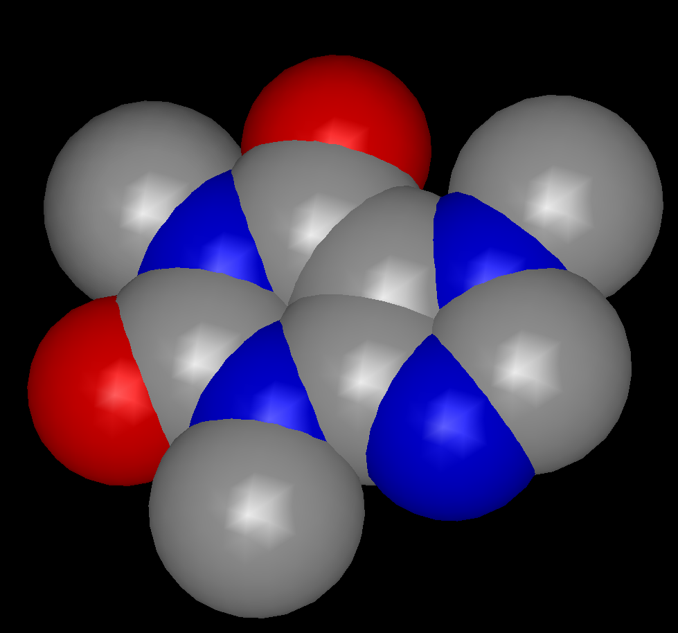
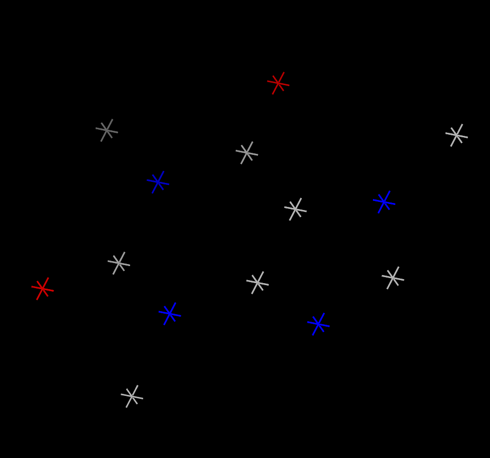
Display Styles
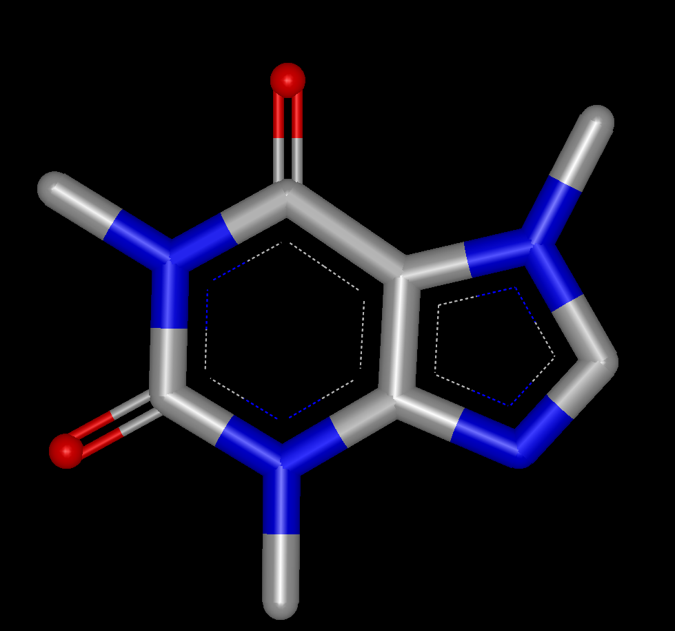
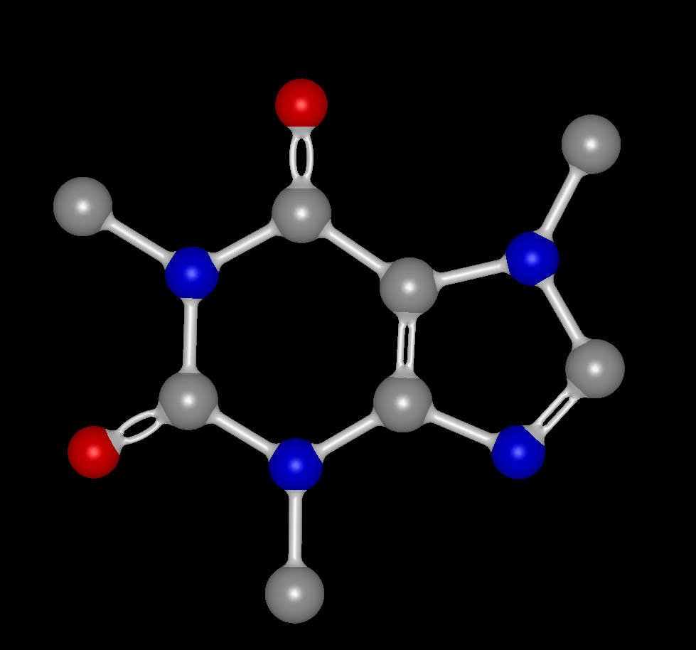
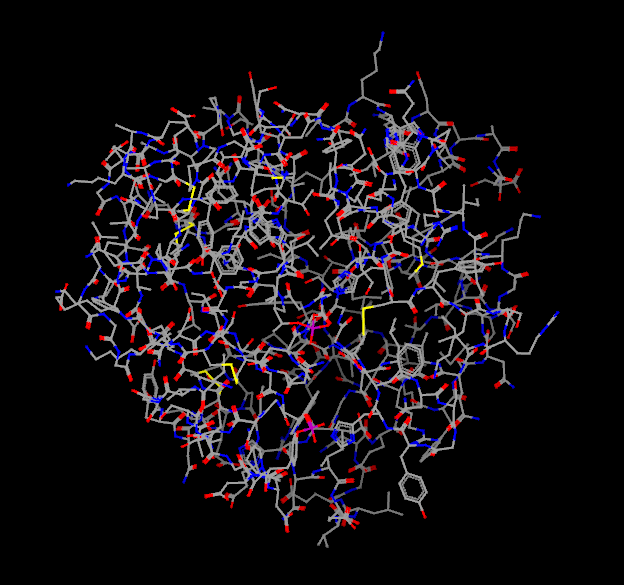
All of the standard molecule display styles are available in VIDA (Wireframe, Stick, Ball and Stick, CPK, and Stars), and are illustrated in Table: Display Styles. By default, small molecules are drawn in Stick mode while large molecules are drawn in Wireframe mode. These defaults can be changed in the application preferences.
|
|
|
|
|
Wireframe |
Stick |
Fancy Ball and Stick |
CPK |
Stars |
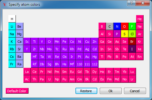
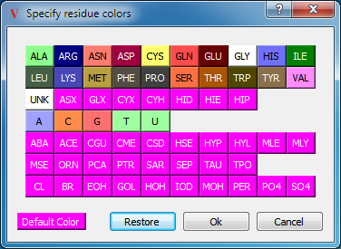
Molecule Color
By default, the atoms in a molecule are colored according to their element types and the bonds in a molecule are colored according to the element types of the two atoms defining that bond. There are two color palettes that specify the actual colors used for a given element, one for use with dark-colored backgrounds and the other for use with light-colored backgrounds. Both of these palettes can be viewed and modified in the application preferences. The dark-background atom color palette can be seen in Table: Color Palettes.
|
|
Atom Color Palette |
Residue Color Palette |
Coloring Schemes
There are a number of molecule specific coloring schemes in addition to the standard element based coloring. The following schemes are discussed below: amino, bfactor, carbon, chain, cpk, cpknew, element, formal charge, group, partial charge, reference, residue, and shapely.
Amino
The amino color scheme is a protein specific scheme which colors atoms according to their individual residues. The residue colors are listed below.
Residue |
Color |
RGB Value |
|---|---|---|
ASP, GLU |
Bright Red |
[230, 10, 10] |
CYS, MET |
Yellow |
[230, 230, 0] |
LYS, ARG |
Blue |
[20, 90, 255] |
SER, THR |
Orange |
[250, 150, 0] |
PHE, TYR |
Mid Blue |
[50, 50, 170] |
ASN, GLN |
Cyan |
[0, 220, 200] |
GLY |
Light Grey |
[235, 235, 235] |
LEU, VAL, ILE |
Green |
[15, 130, 15] |
ALA |
Dark Grey |
[200, 200, 200] |
TRP |
Purple |
[180, 90, 180] |
HIS |
Pale Blue |
[130, 130, 210] |
PRO |
Flesh |
[220, 150, 130] |
Others |
Tan |
[190, 160, 110] |
BFactor
The bfactor color scheme is a protein specific scheme which colors atoms according to the bfactor value using a fixed blue-to-red gradient between 0 and 60.
Carbon
The carbon color scheme colors all of the carbon atoms in the current scope the same color which is specified by the user.
Chain
The chain color scheme is a macromolecule specific scheme which assigns a unique color to each of the macromolecular chains.
CPK, CPKNew
The CPK color scheme is an element specific scheme based on the colors used in the popular CPK plastic space filling models. The CPKnew color scheme is a variant on the CPK color in that it uses a slightly brighter version of some of the colors. The atom colors are listed below with the RGB values for CPK in the third column and the RGB values for CPKNew in the fourth column (if different).
Element |
Color |
CPK: RGB Values |
CPKNew: RGB Values |
|---|---|---|---|
H |
White |
[255, 255, 255] |
|
He |
Pink |
[255, 192, 203] |
|
Li |
Fire Brick |
[178, 34, 34] |
[178, 33, 33] |
B,Cl |
Green |
[0, 255, 0] |
|
C |
Light Grey |
[200, 200, 200] |
[211, 211, 211] |
N |
Sky Blue |
[143, 143, 255] |
[135, 206, 235] |
O |
Red |
[255, 0, 0] |
|
F,Si,Au |
Golden Rod |
[218, 165, 32] |
|
Na |
Blue |
[0, 0, 255] |
|
Mg |
Forest Green |
[34, 139, 34] |
|
Al,Ca,Ti,Cr,Mn,Ag |
Dark Grey |
[128, 128, 144] |
[105, 105, 105] |
P,Fe,Ba |
Orange |
[255, 165, 0] |
[255, 170, 0] |
S |
Yellow |
[255, 200, 50] |
[255, 255, 0] |
Ni,Cu,Zn,Br |
Brown |
[165, 42, 42] |
[128, 40, 40] |
I |
Purple |
[160, 32, 240] |
|
Unknown |
Deep Pink |
[255, 20, 147] |
[255, 22, 145] |
Element
The element color scheme is the default color scheme used when coloring molecules. Colors are assigned according to atomic number. The actual colors used for a given element can be edited in the application preferences as seen in Table: Element Color Palettes.
Element |
Color |
RGB Values |
|---|---|---|
H |
White |
[255, 255, 255] |
C |
Grey |
[180, 180, 180] |
N |
Blue |
[0, 0, 255] |
O |
Red |
[255, 0, 255] |
F |
Green |
[0, 255, 0] |
P |
Magenta |
[192, 0, 192] |
S |
Yellow |
[255, 255, 0] |
Cl |
Lime Green |
[170, 255, 0] |
Br |
Dark Red |
[170, 0, 0] |
I |
Dark Orange |
[170, 85, 0] |
Group I |
Cyan |
[0, 255, 255] |
Group II |
Light Blue |
[160, 160, 255] |
Transition Metals |
Purple |
[170, 0, 255] |
Others |
Pink |
[255, 0, 128] |
Formal Charge
The formal charge color scheme colors atoms according to their formal charge using a fixed red-to-blue gradient between -4 and +4.
Group
The group color scheme is a macromolecule specific scheme which colors each atom according to its position in a macromolecular chain. The colors are assigned along a smooth rainbow spectrum from blue, through green, yellow and orange to red.
Partial Charge
The partial charge color scheme colors atoms according to their partial charge using a red-to-blue gradient between -1.0 and +1.0.
Reference
The reference color scheme colors all of the carbon atoms in the current scope using the current Reference color which can be set in the application preferences. The default is green.
Residue
The residue color scheme is a protein specific scheme which colors atoms according to their individual residues. The actual colors used can be edited in the application preferences as seen in Table: Color Palettes. The default colors correspond to those used in the shapely color scheme.
Shapely
The shapely color scheme is a protein specific scheme which colors atoms according to their individual residues. This scheme is based upon Bob Fletterick’s “Shapely Models”([Fletterick-1982]). The residue colors are listed below.
Residue |
Color |
RGB Values |
|---|---|---|
ALA |
Medium Green |
[140, 255, 140] |
GLY |
White |
[255, 255, 255] |
LEU |
Olive Green |
[ 69, 94, 69] |
SER |
Medium Orange |
[255, 112, 66] |
VAL |
Light Purple |
[255, 140, 255] |
THR |
Dark Orange |
[184, 76, 0] |
LYS |
Royal Blue |
[ 71, 71, 184] |
ASP |
Dark Rose |
[160, 0, 66] |
ILE |
Dark Green |
[0, 76, 0] |
ASN |
Light Salmon |
[255, 124, 112] |
GLU |
Dark Brown |
[102, 0, 0] |
PRO |
Dark Grey |
[ 82, 82, 82] |
ARG |
Dark Blue |
[0, 0, 124] |
PHE |
Olive Grey |
[83, 76, 66] |
GLN |
Dark Salmon |
[255, 76, 76] |
TYR |
Medium Brown |
[140, 112, 76] |
HIS |
Medium Blue |
[112, 112, 255] |
CYS |
Medium Yellow |
[255, 255, 112] |
MET |
Light Brown |
[184, 160, 66] |
TRP |
Olive Brown |
[79, 70, 0] |
ASX,GLX,PCA,HYP |
Medium Purple |
[255, 0, 255] |
A |
Light Blue |
[160, 160, 255] |
C |
Light Orange |
[255, 140, 75] |
G |
Medium Salmon |
[255, 112, 112] |
T |
Light Green |
[160, 255, 160] |
Backbone |
Light Grey |
[184, 184, 184] |
Special |
Dark Purple |
[94, 0, 94] |
Default |
Medium Purple |
[255, 0, 255] |
Proteins
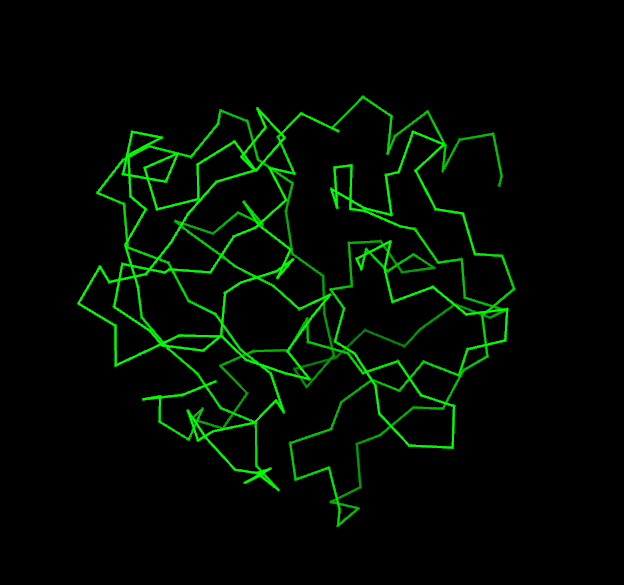
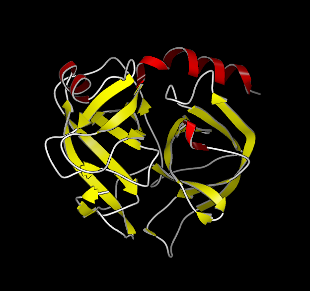
In addition to the standard display styles, the two protein specific displays of C-Alpha Traces and Ribbons are supported. Examples of these display styles can be seen in Table: Protein Styles.
|
|
|
Wireframe |
C-Alpha Trace |
Ribbon |
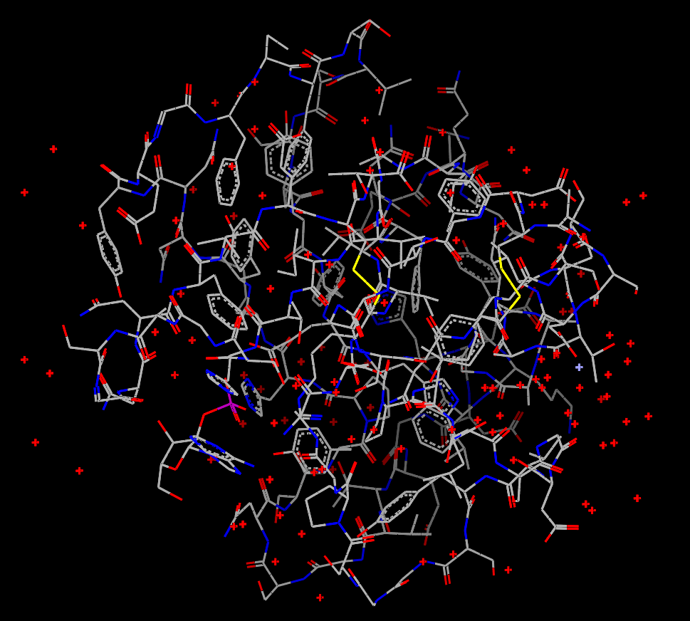
Given that protein files often inevitably contain many extra components that are not necessarily of interest to the user (waters for example), the ability to hide the display of non-bonded atoms is provided to ease the viewing of proteins without having to manually edit the input file. An example of a protein displayed with and without waters can be seen in Table: Water Styles. There is also a button in the style panel of the Style Control window that will toggle the display of non-bonded atoms.
|
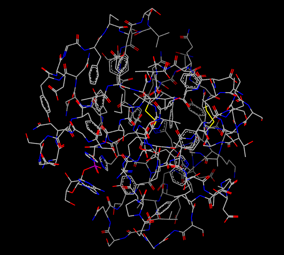
|
Protein with waters |
Protein without waters |
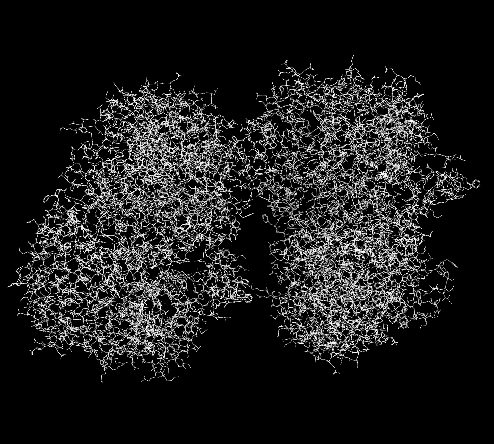
|
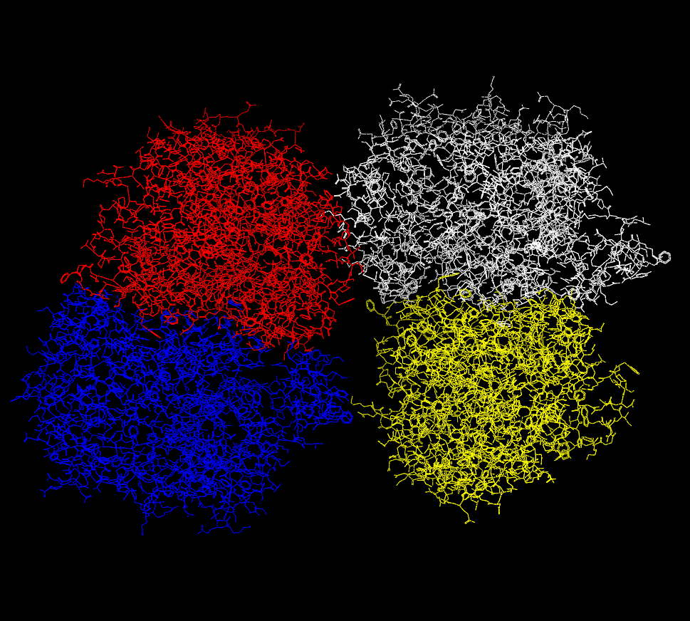
|
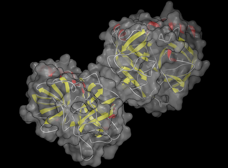
Multimer displayed as a single molecule |
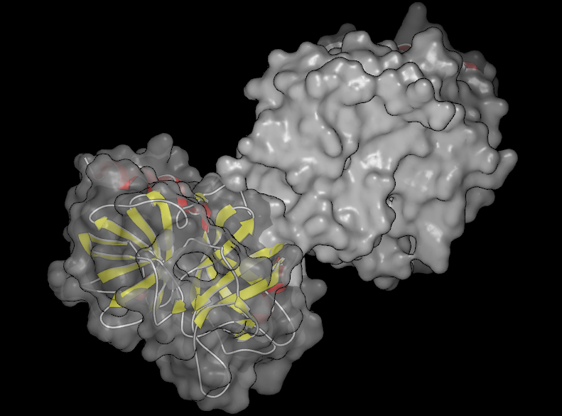
Multimer displayed as multiple molecules |
Another common scenario when working with proteins is that the input file contains a large multimer which, as expected, is interpreted as a single molecule. However, sometimes the ability to interact with the individual components is of particular value. The ability to split a molecule into separate components can be performed by selecting the “File > New Molecule > From Split > Components” menu option. This function will then determine what the individual components of the Focused molecule are and create a new list containing a new molecule for each component. The original molecule is not changed or deleted. An example of this process can be seen in Figure X.Y. The From Split submenu also contains “Selected” and “Marked” options which will create new molecules from the original based on the selected or marked set of atoms.
It may also be of interest to put some of these components back together into a single molecule. This can be done by choosing one of the following options from the “File > New Molecule > From Merge” submenu: “Selected”, “Marked”, “Visible”. Choosing any one of these options will create a new molecule which is composed of all the molecules that were either “Selected”, “Marked”, or “Visible” at the time of the operation.
Monitors
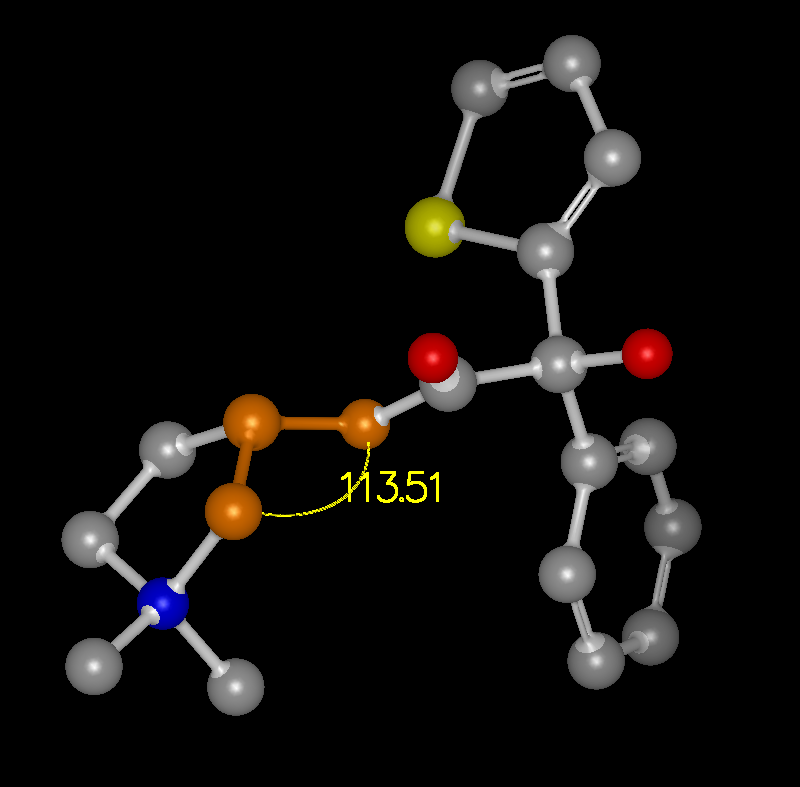
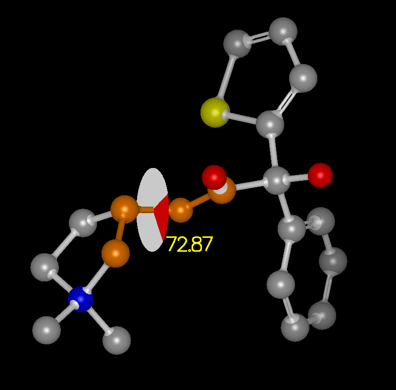
The ability to display measurement monitors is a useful feature and is well supported. Access to these measurement facilities is available from the Mouse toolbar on the left hand side of the 3D display. There is a single button with three options which turn on Distance, Angle, and Torsion measurement respectively.
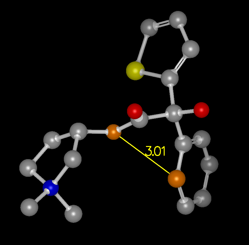
|
|
|
Distance Monitor |
Angle Monitor |
Torsion Monitor |
When the mouse is put into one of these modes, the measurements are made based on the selected set of atoms. In Distance mode, the first atom selected is consider the “anchor” atom. Once the anchor atom has been selected, a temporary distance monitor will be displayed to any other atom that the mouse passes over. Selecting another atom will create a permanent monitor and clear the anchor. In Angle mode, the first two atoms selected are considered the anchor atoms and a temporary angle monitor will be displayed to any other atom that the mouse passes over. Selecting a third atom will create a permanent monitor and clear the anchors. In Torsion mode, the first three atoms selected are considered the anchor atoms and a temporary torsion monitor will be displayed to any other atom that the mouse passes over. Selecting a fourth atom will create a permanent monitor and clear the anchor.
Monitors can be removed by selecting the monitor of interest and then choosing the “Delete” option in the right-click menu. All of the visible monitors can be deleted in one step by right-clicking in the 3D display and selecting the “Delete visible monitors” option. Monitors are also displayed in the “List Window” and can be deleted individually there. Examples of the three types of monitors can be seen in Table: Monitor Types.
Monitors serve an important role when in editing mode as the properties they measure can be modified by selecting the monitor and then using the mouse wheel to adjust the value up or down. By default, the smaller portion of the associated molecule will be the part that is moved. This can be reversed by holding down the Ctrl key while using the mouse wheel. To achieve fine control of the values, hold down the Shift key while using the mouse wheel.
Hydrogen Bonds
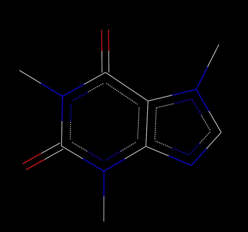
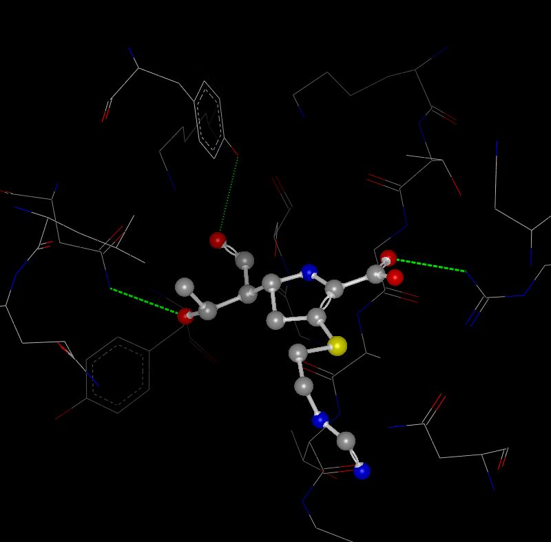
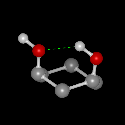
Both internal (intramolecular) and external (intermolecular) hydrogen bonds can be displayed. Hydrogen bonds are determined by typing all of the atoms as either acceptors, donors, both, or neither. Then the hydrogen bond energy is calculated between all acceptors and donors based on the ChemScore scoring function which takes into account both interatomic distance as well as the coordination geometry ([Eldridge-1997]). This function provides a relative score between 0 and 1.0 for the energy of the hydrogen bond. For all hydrogen bonds with an energy greater than 0, the bond is drawn as a dotted green line. The thickness of the line as well as the spacing between the dots correlates to the bond energy. Therefore, thicker more solid lines have higher energy than thinner more dotted lines. An example of both internal and external hydrogen bonds can be seen in Table: Hydrogen Bonds.
|
|
External Hydrogen Bonds |
Internal Hydrogen Bonds |
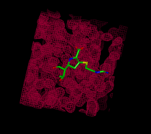
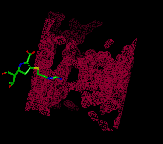
Grid Visualization
Grids are spatial arrays of data that are sampled at regular intervals. Grids may contain electrostatic samples of spatial regions, density samples, and other potential fields.
A grid can have a variable number of contours. Each contour has an index starting at 1 for the first contour. Additionally, every contour has its own individual color and a threshold value which can be positive or negative (also known as the “contour level”). There are three different display styles for grids contours: Solid, Mesh and Cloud.
Grid Types
As mentioned in the previous section, there are multiple different predefined grid types that are supported including: Electrostatic, ET, FRED, Generic, Difference Map, and Regular Map.
Electrostatic
Electrostatic grids are the only type of grid that can be actually be generated within VIDA as opposed to simply being visualized. Electrostatic grids are created for individual molecules using OpenEye’s Zap toolkit (for more information, please see the Zap toolkit documentation). The creation of the grid requires the presence of partial charges on the input molecule. If partial charges were already present on the molecule, those will be used in the calculation. However, if no partial charges were present (or the user decides to ignore them, which can be set in the application preferences), temporary partial charges will be calculated using MMFF94 or AM1-BCC ([Jakalian-2000], [Jakalian-2002]). If a molecule has greater than 50 atoms, MMFF94 charging will be done even if AM1-BCC was selected. However, for proteins an alternate residue based charging model is available and can be selected in the preferences. This model assigns partial charges based on residue information as is shown below:
Residue |
Residue Atom |
Partial Charge |
|---|---|---|
ASP |
OD1, OD2 |
-0.5 |
GLU |
OE1, OE2 |
-0.5 |
LYS |
NZ |
+1.0 |
ARG |
NE |
+1.0 |
The grid spacing is dynamically determined based on the number of atoms in the input molecule. However, it is possible to specify a fixed spacing in the grid preferences. Be warned, however, that specifying very fine spacings (< 2.0 Angstroms) may consume a surprisingly large amount of memory, (in some cases more than may be available on the computer), which can lead to program failure. This should be considered a very advanced feature to be used only when necessary and when all other data has been saved. Finally, it has been observed in research at OpenEye that adding salt to the electrostatic calculation has a beneficial effect on the grids generated. The salt concentration can be specified in the preferences. The default concentration is 0.04 M. The maximum concentration that can be specified is 0.1 M.
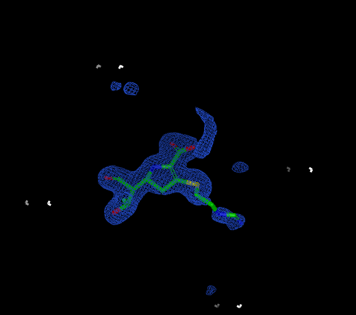
Electrostatic grids (as well as ET grids) are special in that they are always generated with two default contours: a positive one and a negative one. These contours cannot be deleted and new contours cannot be added. The positive contour is colored blue by default and the negative contour is colored red. The contour levels of the two contours are coupled together and so changing one will change the other.
ET
ET (or Electrostatic Tanimoto) grids are generated by OpenEye’s BROOD and EON applications. When viewed in VIDA they behave, and are treated essentially the same, as Electrostatic grids.
FRED
FRED grids are shape potential grids that are created by OpenEye’s FRED application. In VIDA, the behave just like Generic grids except that their default contour color is purple instead of blue.
Generic
Generic grids are effectively the most basic grids and act as the primary grid workhorses. They are completely customizable and have bare-bones settings. They default to having just one contour with a default color of blue. Additional contours can be added as well as removed. These default values can be changed in the Grids section of the application preferences.
Reentrant Grids
|
|
|
Infinite grid |
Infinite grid rendered at a different center |
Non-reentrant grid |
Some grids have fixed extents and some grids are infinitely reentrant in space. Reentrant grids obviously cannot be displayed in their entirety, so instead only the region around the center of the current scene is displayed. Grids that are being rendered as reentrant can be distinguished from non-reentrant grids by the absence of grid corners which define the extents of non-reentrant grids.
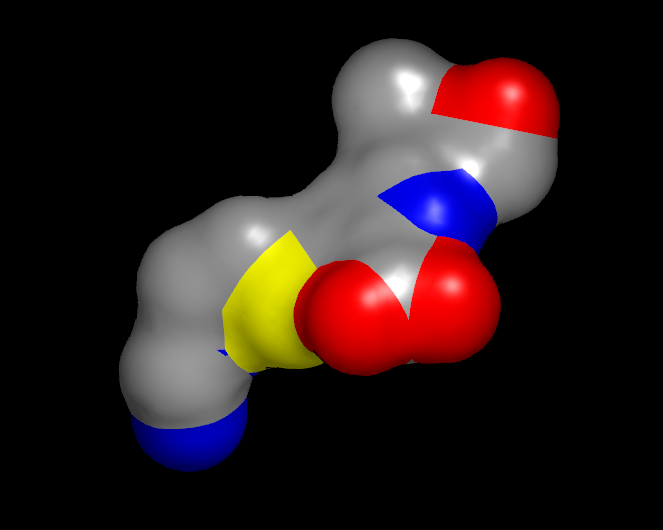
Surface Visualization
Surfaces are infinitely thin three dimensional connected regions that represent objects such as molecular or accessible surfaces of molecules. Surfaces can be selected (or scribed), cropped, colored, and made transparent in part or in whole.
Display Styles
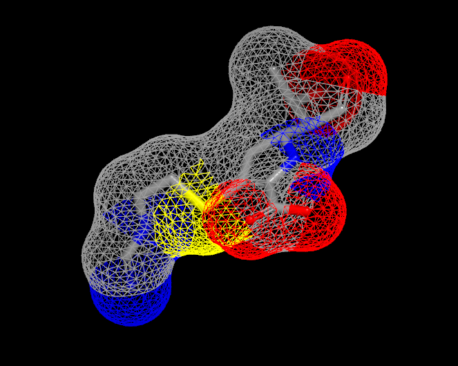
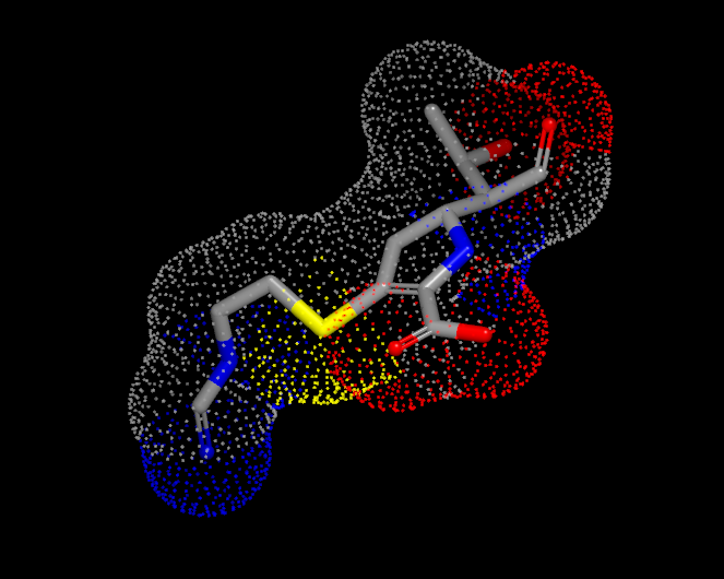
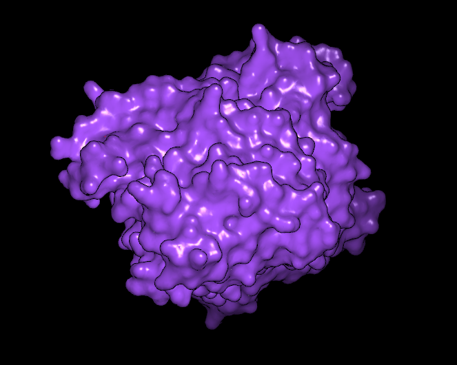
Surfaces can be visualized in one of three display styles: Solid, Mesh, and Points. These individual display styles can be seen in Table: Surface Styles.
|
|
|
Solid |
Mesh |
Point |
Surface Color
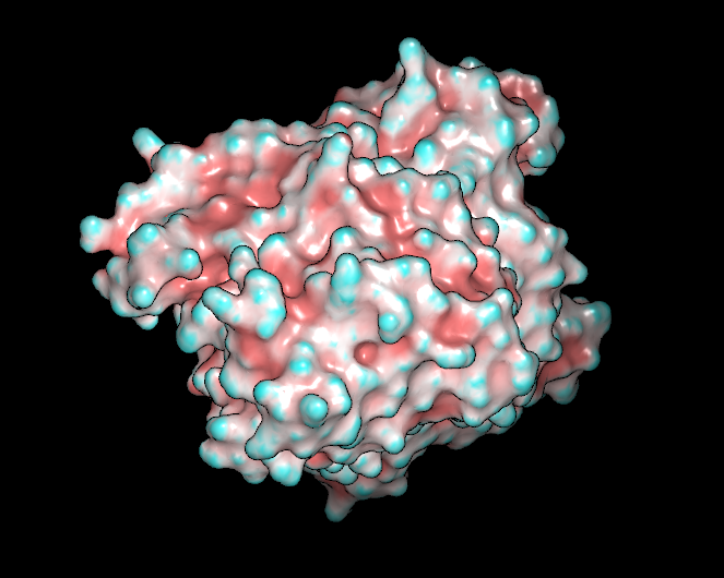
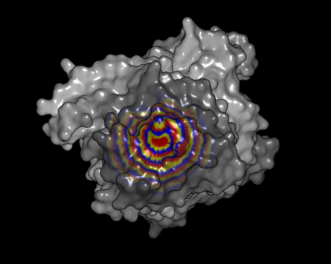
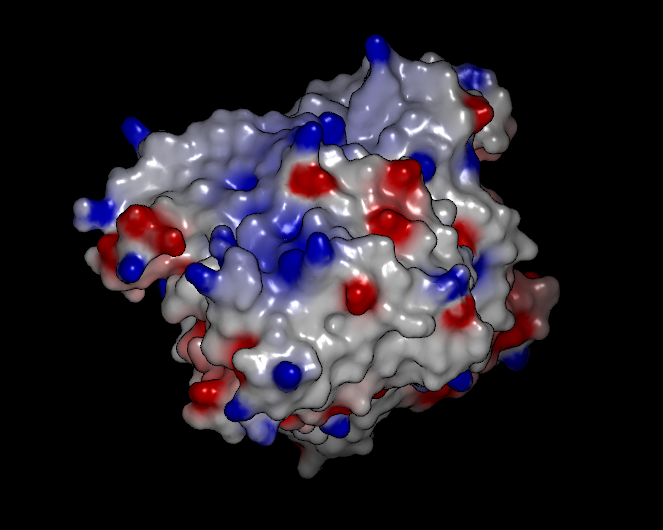
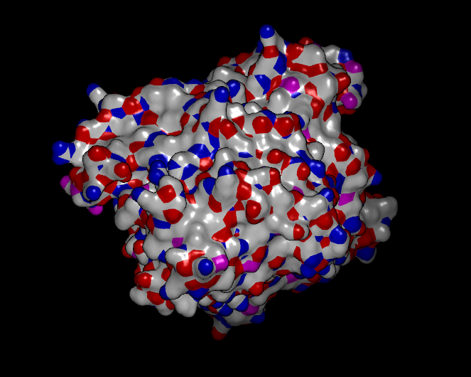
There are a number of surface specific coloring schemes in addition to the standard single color scheme and some examples are illustrated in Table: Surface Colors. The following schemes are discussed below: atom color, curvature, distance, electrostatics, grid, hydrogen bond potential, hydrophobicity, and surface potential.
|
|
|
Single color |
Color by atom |
Color by curvature |
|
|
|
Color by distance |
Color by electrostatics |
Color by hydrogen bond potential |
|
||
Color by hydrophobicity |
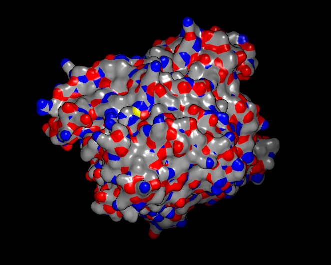
Atom Color
The atom color scheme colors each vertex on the surface using the color of the nearest atom to that vertex in the molecule that the surface was created from (see Table: Surface Colors). This scheme will not work if the surface was not created from a molecule and also if that molecule is not currently present.
Curvature
The curvature scheme colors each vertex on the surface according to the curvature of the surface at that vertex using a pink-to-cyan gradient where cyan indicates high convexity and pink indicates high concavity (see Table: Surface Colors).
Distance
The distance scheme colors each vertex by its distance from either the selected set of atoms or the visible set of atoms (if none are selected at the time of coloring). Each band of color represents a distance of one Angstrom from the selected set. The color banding is continuously repeated as the distance increases, but the colors fade to white with each repetition to show the distance effect (see Table: Surface Colors).
Electrostatics
The electrostatics scheme colors each vertex on the surface according to the electrostatic potential at that vertex using a red-to-blue gradient from -7.0 to +10.0 (see Table: Surface Colors). This range can be changed if desired in the application preferences in the Surfaces section.
The electrostatic potential at the surface is calculated using OpenEye’s Zap toolkit (for more information, please see the Zap toolkit documentation). By default, VIDA will use the molecule’s input partial charges in the calculation (if any were specified). However, if no partial charges were specified, VIDA will assign partial charges using either MMFF94 (the default) or AM1-BCC. The choice of charge model can be specified in the application preferences. If a molecule has greater than 50 heavy atoms, MMFF94 will always be used in place of AM1-BCC regardless of the set preferences.
Proteins have an alternative charging option based on residue information. The charge model can be seen in the table below. This model is used by default (if no partial charges were specified), but it can be disabled in the application preferences.
Residue |
Residue Atom |
Partial Charge |
|---|---|---|
ASP |
OD1, OD2 |
-0.5 |
GLU |
OE1, OE2 |
-0.5 |
LYS |
NZ |
+1.0 |
ARG |
NE |
+1.0 |
Grid
The grid scheme colors each vertex on the surface according to the grid potential at that vertex using a red-to-blue gradient from the minimum grid value to the maximum grid value. The grid potential is determined by mapping the specified grid onto the surface.
Hydrogen Bond Potential
The hydrogen bond potential scheme colors each surface vertex according to the hydrogen bond class (Acceptor=Red, Donor=Blue, Both=Magenta) of the nearest atom in the surface’s molecule (see Table: Surface Colors). This scheme will not work if the surface was not created from a molecule and also if that molecule is not currently present.
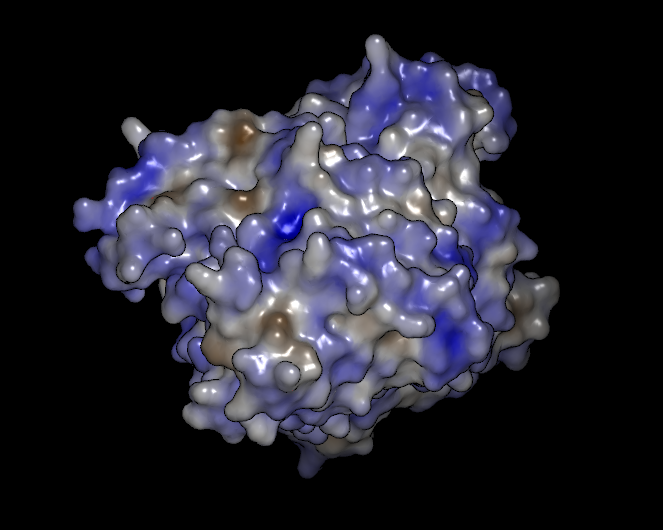
Hydrophobicity
The hydrophobicity scheme colors each vertex according to a specified hydrophobic color scale based on the OEXLogP values of the underlying atoms. More hydrophobic areas are brown, while more hydrophilic areas are blue. This scheme will not work if the surface was not created from a molecule or if that molecule is not currently present.
Surface Potential
The surface potential scheme colors each vertex according to the potential value at that vertex using a red-to-blue gradient from the surface potential minimum to the surface potential maximum. This scheme differs from the electrostatic scheme in that the coloring is based on the stored potential values as opposed to calculated potential values. Typically, surfaces generated within VIDA will not have any stored potential values. However, surfaces created externally using OpenEye’s Spicoli toolkit, for example, can store values in the potential field and as such can be colored accordingly.
Selection
For surfaces created from molecules, the minimum selectable part is the surface corresponding to a single atom. A line of atom surfaces can be selected by selecting one spot on a surface and then by holding down the Shift key when selecting another. This starting selection can be grown (and shrunk) using the Selection pane in the Style Control. Double-clicking on the surface will select the entire surface. For surfaces created without a molecule (usually outside of VIDA), the minimum selectable part of a surface is a single vertex, and the above operations work on vertices instead of atoms.
Symmetry
VIDA supports symmetry operations. This support includes a submenu under the Edit menu which controls displaying symmetry in the 3D window, and some items in the popup menu of the list window which allow setting or editing symmetry parameters.
Symmetry information may be read from certain files. When VIDA reads
PDB-format files which have valid CRYST1 records, symmetry information is
taken from that record for all molecules read from that file. Similarly,
when VIDA reads MTZ-format reflection files the symmetry information
is read from that file and, of course, VIDA will read symmetry
information if it is present in an .oeb file.
When symmetry display is enabled, all symmetry operators which would result in a molecule within a certain distance (the symmetry radius) of the screen center are displayed. This means that as the view is translated, certain symmetry replicates will appear and disappear as they move into or out of the symmetry zone. There is, therefore, no need to manually re-calculate the symmetry after translating the model.