Tutorial 3: NGS and Sanger Pipeline with Automated Top Lead Selection (PacBio), In-Vitro Library

Background

See Background from Tutorial 1

This is one of the most comprehensive Floes available. The goal of this tutorial is to utilize the automated selection pipeline for lead selection using both NGS and Sanger datasets simultaneously. We will use the analyze tool to identify the overlap population (see description under overlap_population :) which includes the Sanger populations.

STEP 1 - Login to Orion, Set-Up Directory, Locate Tutorial Files

1. Follow Step 1 from Tutorial 1, #1-2.

2. Find these two additional SANGER input files:

   D) Organization Data / OpenEye Data / Tutorial Data / AbXtract / SANGER_aa.xlsx

   E) Organization Data / OpenEye Data / Tutorial Data / AbXtract / scaffold_ref_db_aa.txt

3. Create a general tutorial directory and tutorial 3 subdirectory under PROJECT DIRECTORY / TUTORIALS / TUTORIAL_3 (This is your BASE DIRECTORY and should be used for all outputs for this Tutorial 3 below).

STEP 2 - Select the ‘NGS and Sanger Pipeline with Automated Top Lead Selection’ Floe

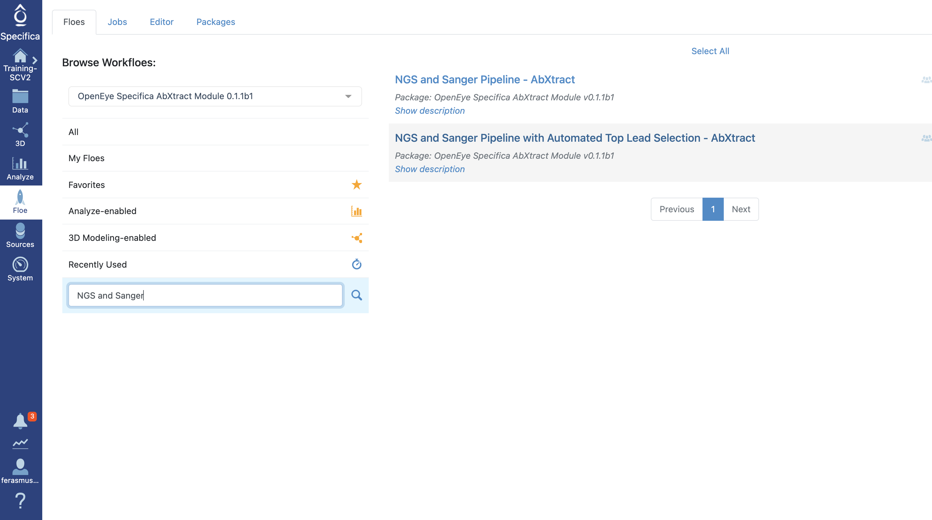
1. Select the tab along the left side tab titled ‘Floe’.

2. Click the ‘Floes’ tab.

3. Choose the ‘OpenEye Specifica AbXtract Module’.

4. Select the Floe ‘NGS and Sanger Pipeline with Automated Top Lead Selection’.

STEP 3 - Prepare Sanger Files

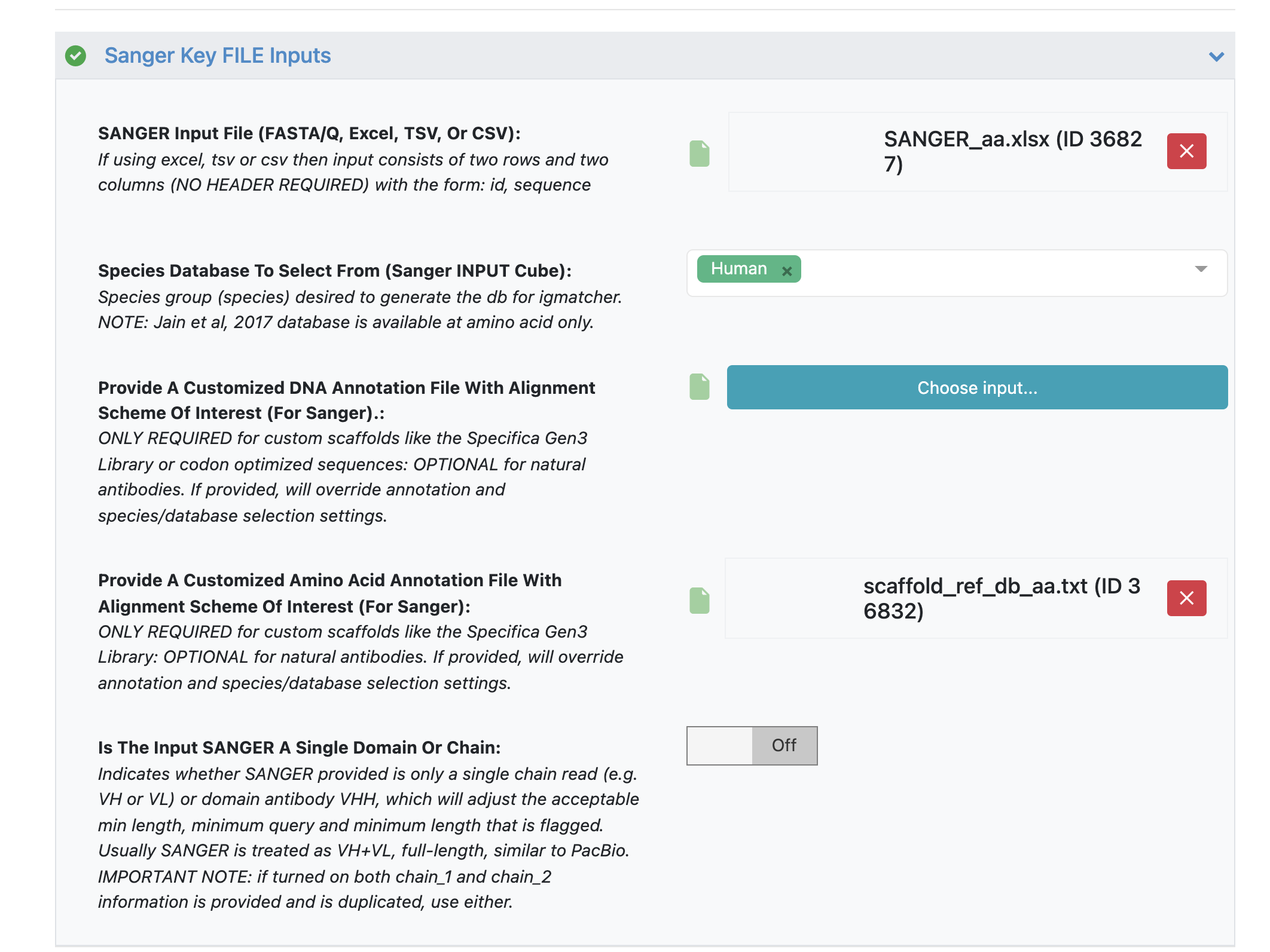
1. Under the ‘Sanger Key FILE Inputs’ load ‘SANGER Input File’ - ‘SANGER_aa.xlsx’.

2. Under parameter option ‘Provide A Customized Amino Acid Annotation File With Alignment Scheme Of Interest’ load the annotation file - ‘scaffold_ref_db_aa.txt’

Important Note

While amino acid sequences work well with the reference database using ‘human’ input, we will still load a custom annotation file to get desired scaffold name for input that matches names used in the custom DNA annotation file ‘scaffold_ref_db_codon_optimized_dna.txt’.

STEP 4 - Prepare PacBio Files and Start Job

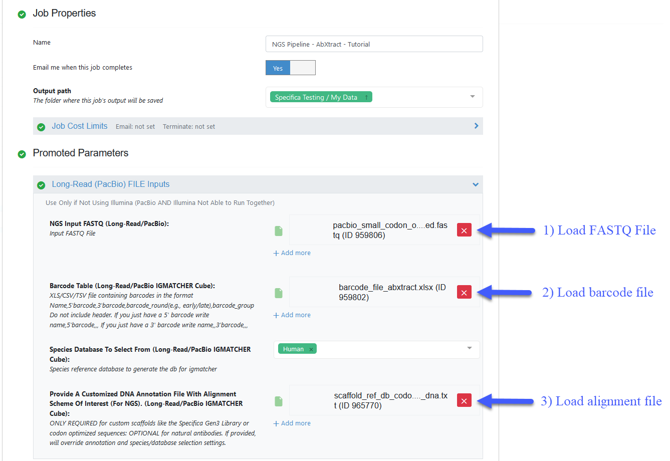
1. Load FASTQ file - ‘pacbio_small_codon_optimized.fastq’.

2. Load barcode XLSX file - ‘barcode_file_abxtract.xlsx’.

3. Load alignment TXT file - ‘scaffold_ref_db_codon_optimized_dna.txt’.

Important Note

All the remaining parameters can be kept as the default values. Scroll through remaining “Promoted” parameters to get a sense of these parameters.

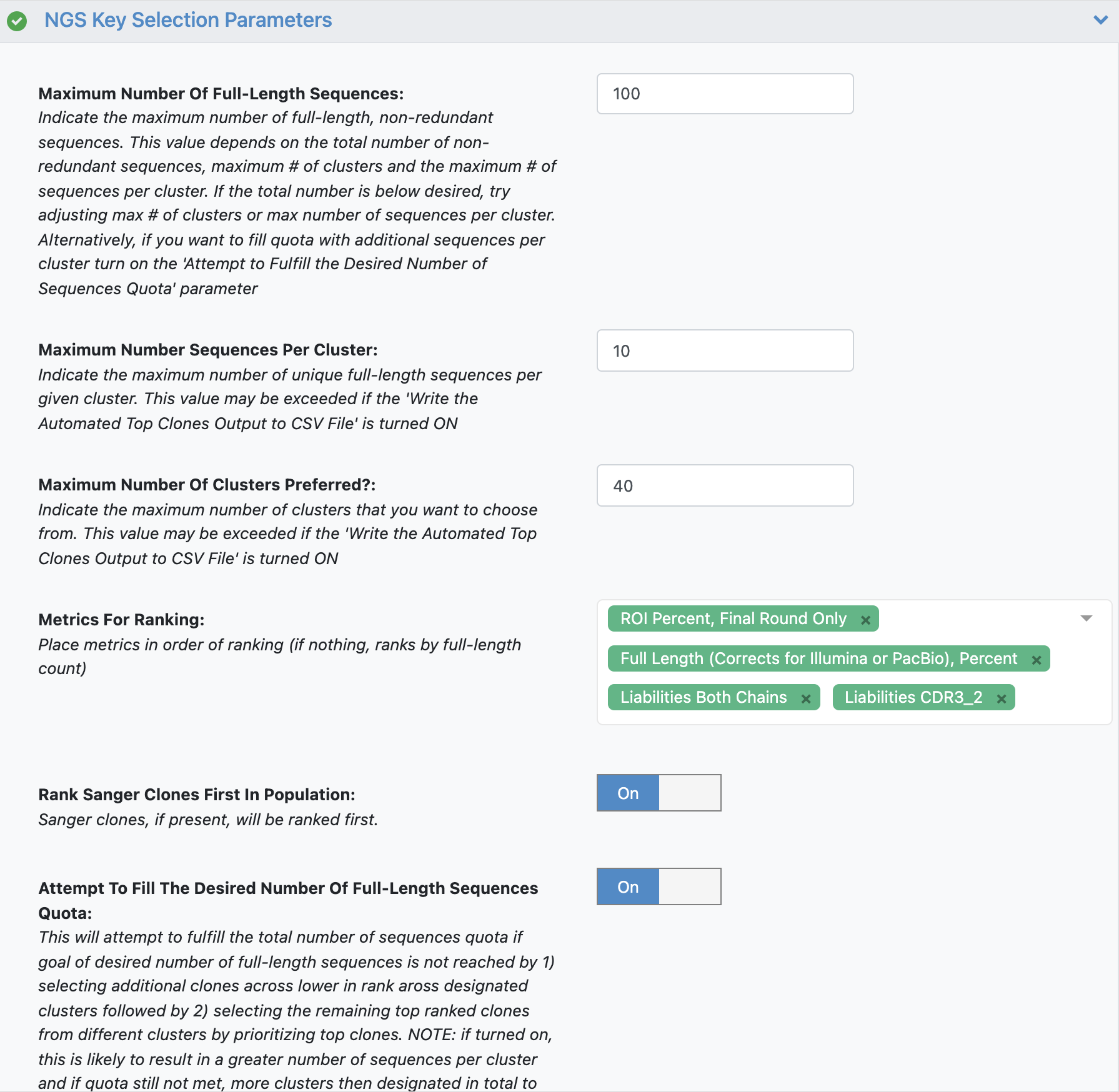
See tutorial 2 automated selection options for more details.

Important Note

The additional parameter ‘Rank Sanger Clones First In Population’ will prioritize any clones identified by Sanger input by identifying clusters associated with these Sanger clones. The automated selection will still select across clusters but will place any Sanger clones at the top of the Metrics For Ranking list.

4. Click ‘Start Job’.

STEP 5 - Open the Floe Report to Get a Detailed Understanding of the Selected or ‘Picked’ Population

1. Under the ‘Jobs’ tab find the ‘NGS and Sanger Pipeline with Automated Top Lead Select’.

2. Click the ‘Show non-dataset files’ checkbox. The breakdown of datasets, collections (Floe reports) and files (CSV) are depicted here:

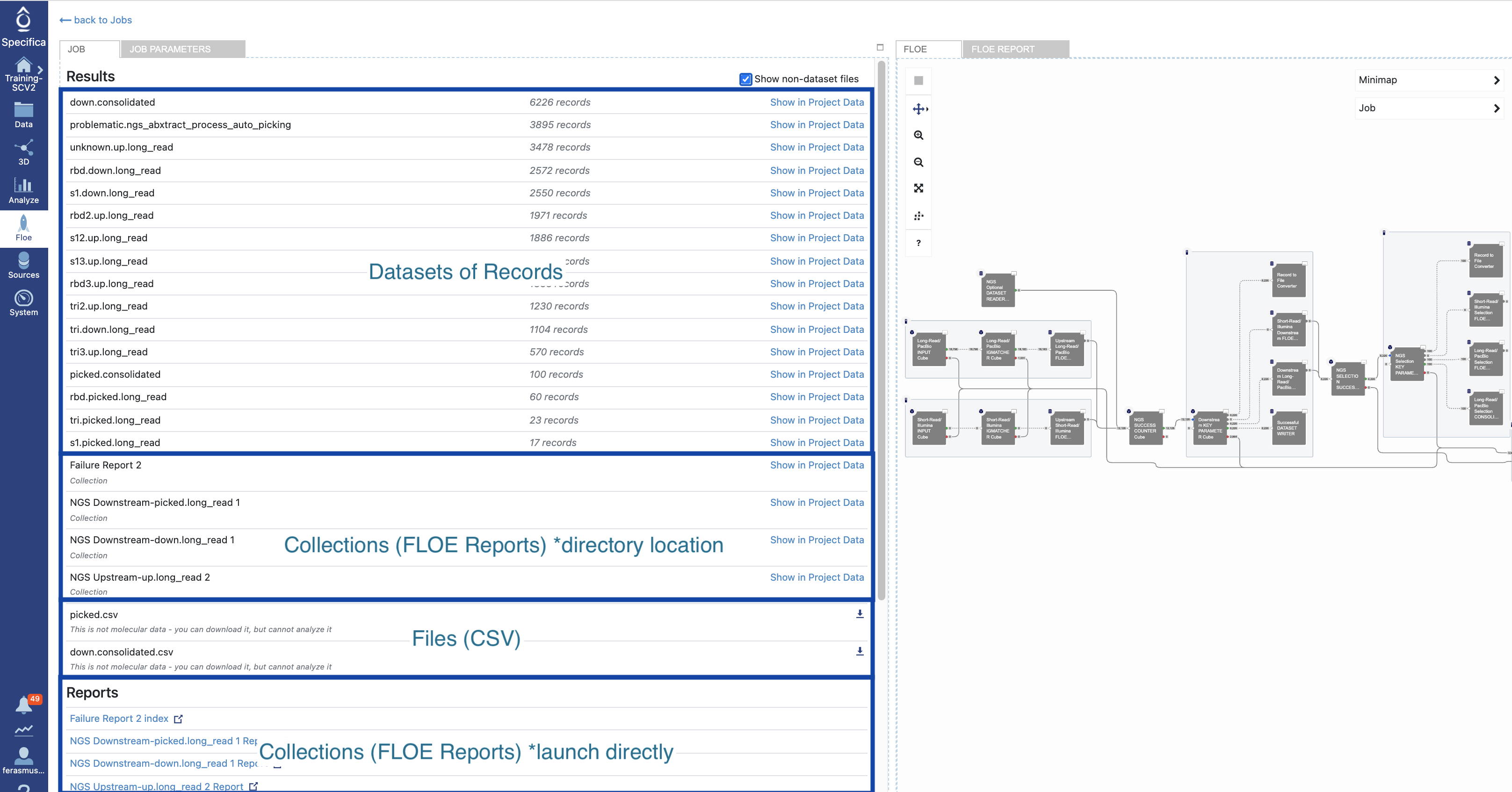
3. Click on the ‘NGS & Sanger Downstream-down.long_read’ under the ‘Reports’ section to launch in browser. Give it some time to load in browser.

4. See the ‘General stats’, which provides a snapshot of the number of non-redundant full-length, LCDR3, HCDR3, LCDR3 and HCDR3 sequences. Chain_1 represents the variable light chain (VL) and chain_2 represents the variable heavy chain (VH). The overlap shows the overlap of the region of interest (HCDR3) across the different populations.

5. See the ‘Cluster/Region of Interest:Sanger’, which indicates the distinct region of interest cluster id (e.g., 76F) and sequence (e.g., H3 sequence) within the Sanger population. These are the Sanger sequences clustered in context of NGS.

6. See the ‘Unique Sequences in NGS or Sanger Outputs Overall’, which provides an overview of the total diversity across different regions of interest that are distinct to Sanger, NGS or in both. Because this is a smaller dataset we do not get complete overlap between NGS and Sanger.

7. In the subpanel (e.g. Group: tri), see the table ‘Downstream NGS Clones by Cluster ID/Region of Interest within Sanger Overlap…’ we can identify the cluster id and corresponding Sanger Sequence ID. These sequence IDs are built off how the user specified the condensing of Sanger sequences (e.g., full-length) and the comma-separated id’s (e.g., 0_Sanger, 155_Sanger, 151_Sanger) indicate those Sanger clones that share the same region of interest as indicated (e.g. HCDR3). We also see the NGS metrics of the given ROI as indicated in the table.

8. Return to Job overview of all the datasets, floe reports and files - see similar reference

9. Find the the dataset titled ‘picked.consolidated’ and ‘Show in Project Data’.

10. Find the ‘picked.consolidated’ in the project directory. Select the Workfloe button.

11. Under Search Bar, search for ‘Subset the Number of Fields for Export’ and click ‘View all Workfloe options’.

12. Keep following fields (for more details, see key fields reference):

    A) seq_id

    B) match_name_1

    C) match_name_2

    D) cdr3_aa_2

    E) sequence_aa_1

    F) sequence_aa_2

    G) cluster

    H) well_id (under Sanger Overlap Fields to Keep)

13. Click ‘Start Job’.

14. Next go back to the data directory and activate the ‘picked.consolidated’ and the ‘down.consolidated’ dataset together.

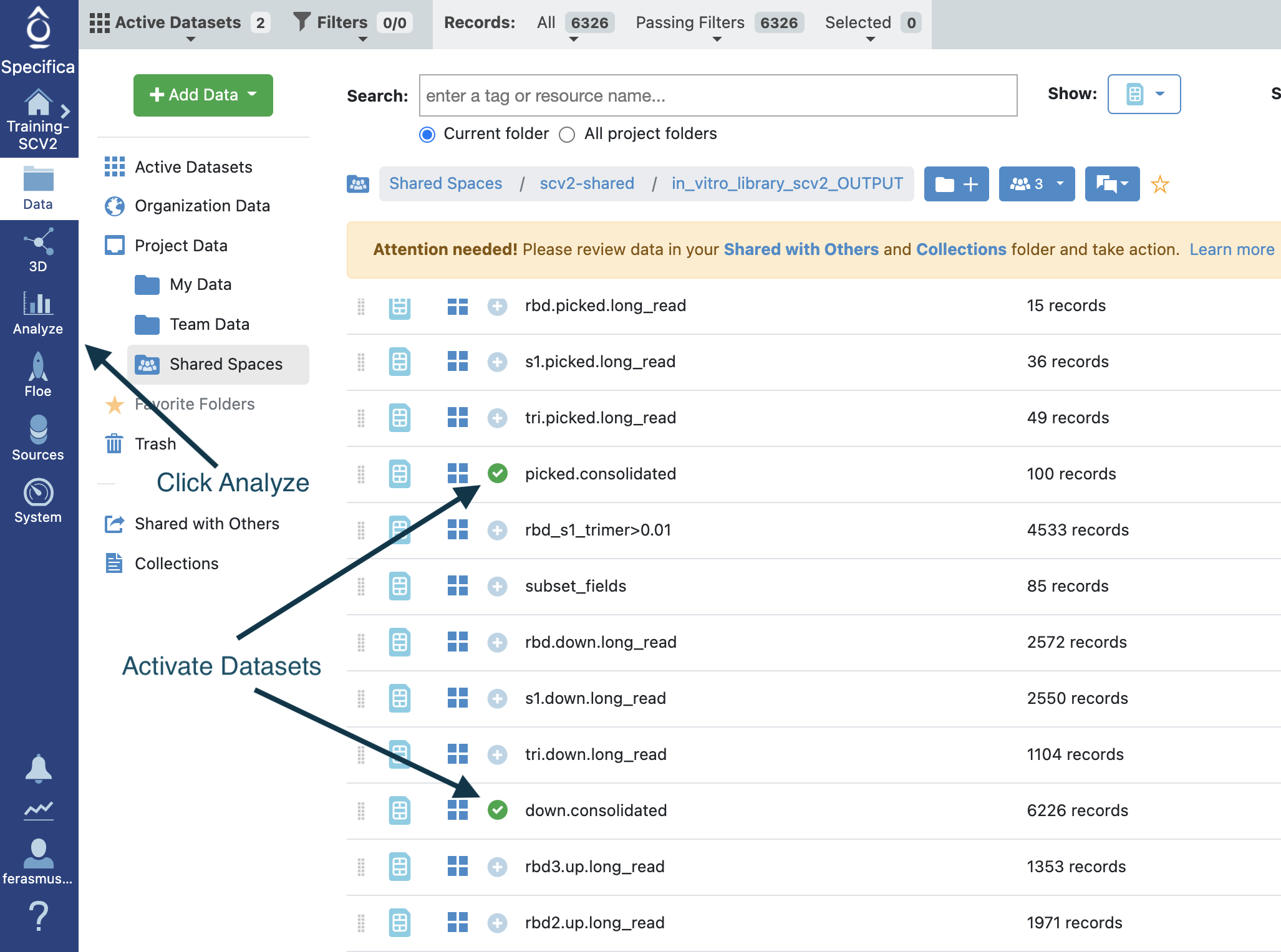
15. Open in the Analyze tool.

STEP 6 - Subset NGS Only Population by Cluster and Overlap_Population

1. Click the Analyze tab to activate the interactive tool.

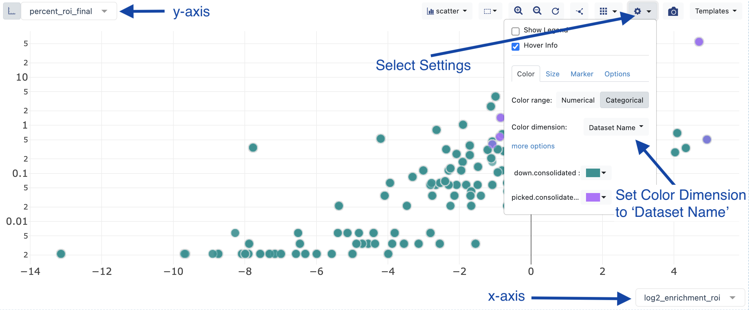
2. select y-axis - percent_roi_final.

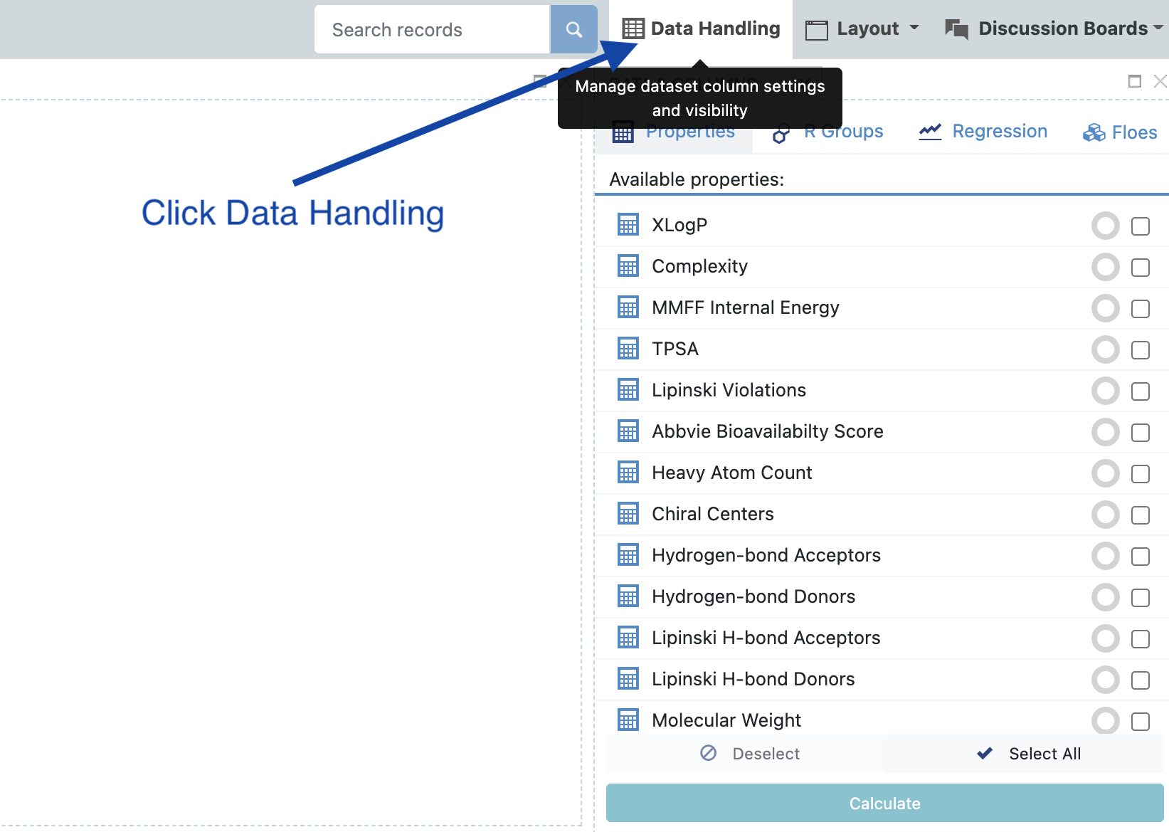
3. Click the ‘Data Handling’ tab near top:

5. Make sure that under ‘Display’ ‘log2_enrichment_roi’ has all options selected (or at least in spreadsheet and plot) and click ‘Apply’.

6. Select x-axis - log2_enrichment_roi.

Important Note

If option not available select ‘count’ to initialize then select the y-axis after data has loaded.

7. Change the color of the records by selecting the plot settings and choosing ‘Dataset Name’.

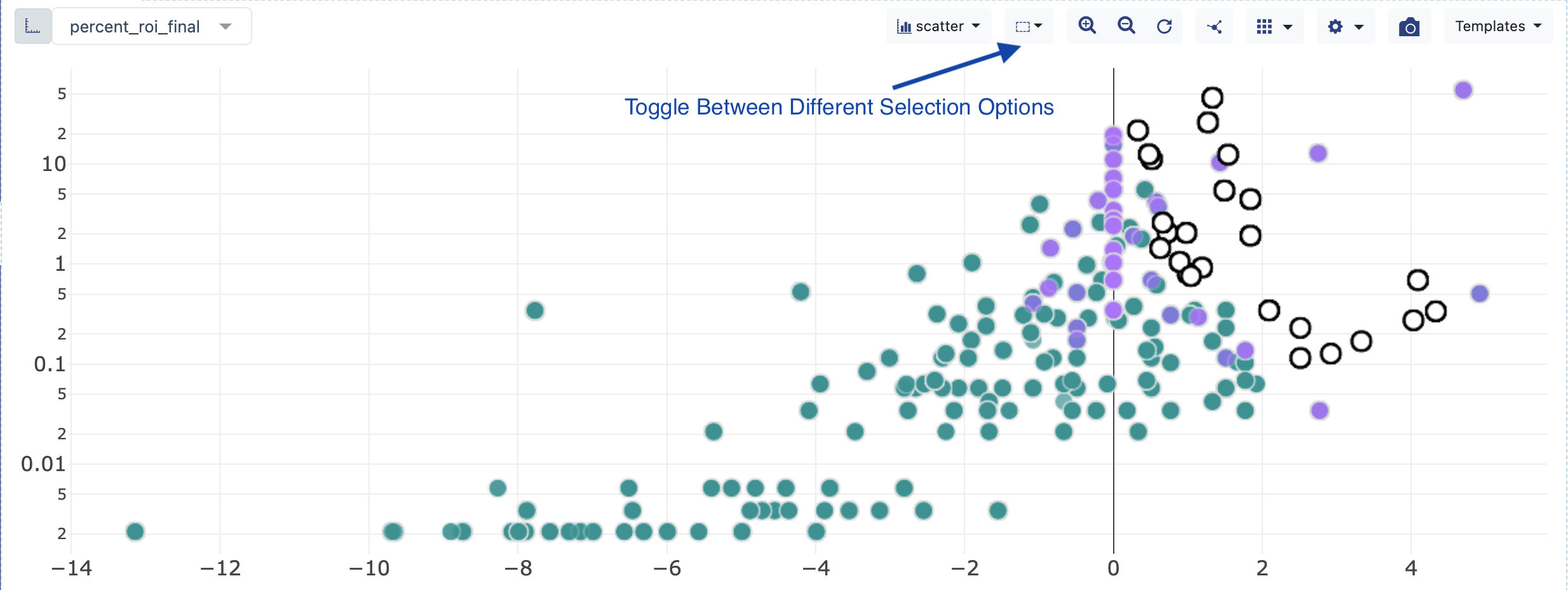
8. Use the Shift key on the keyboard to select any remaining Non-Picked Populations that are highly enriched in population. Toggle between lasso and rectangle select.

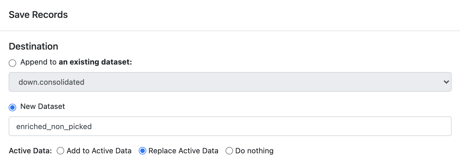
9. With the selected population click the ‘Selected’ option near the top > click ‘Save Records’ > ‘New Dataset’ > provide a name ‘enriched_non_picked’ and > ‘Replace Active Data’.

10. Allow the new dataset loads into the interactive interface. If it does not load properly, remove all active datasets, find ‘enriched_non_picked’ dataset in project directory, make active, and reload in Analyze.

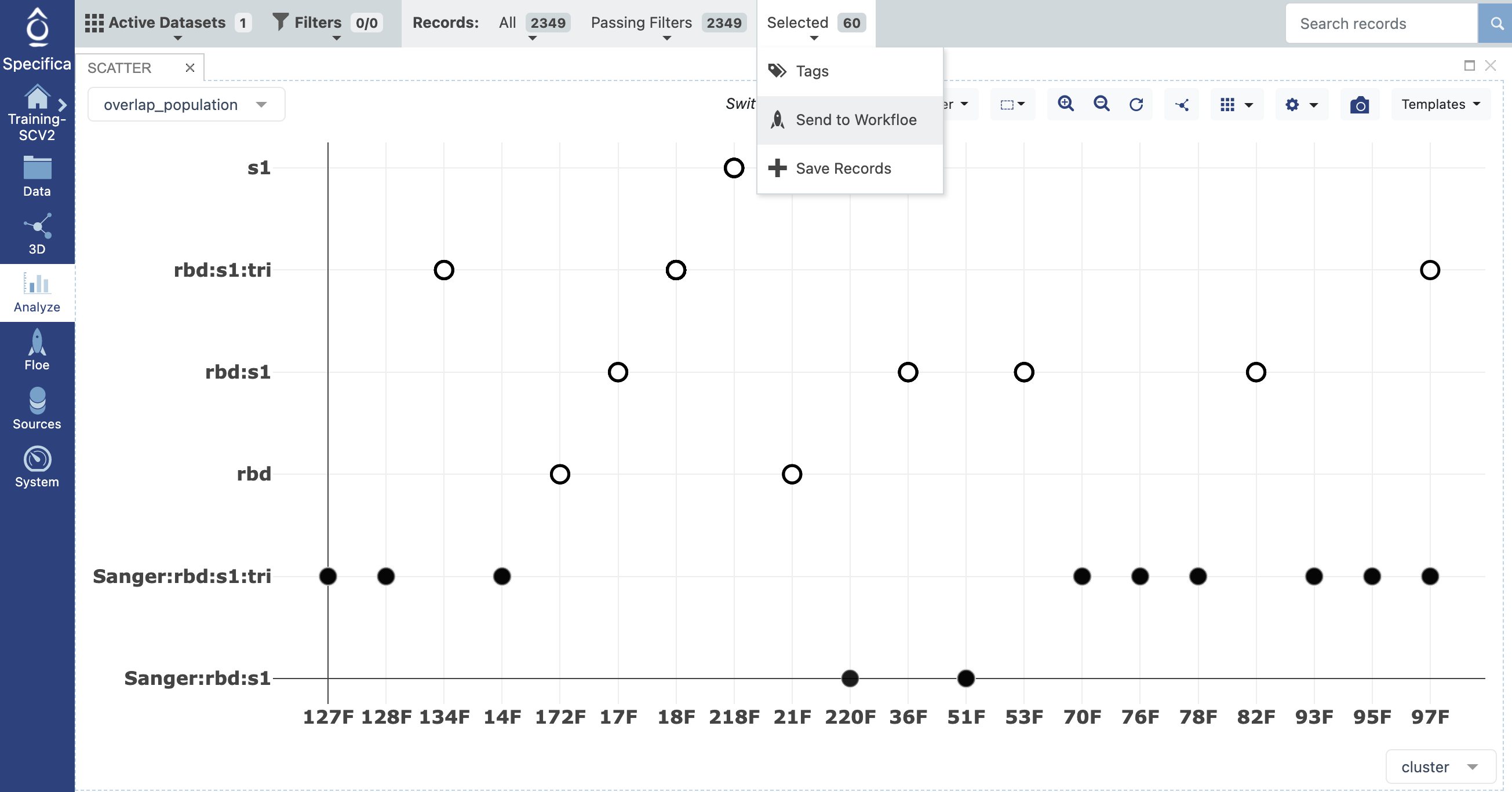
11. set x-axis - cluster.

12. set y-axis - overlap_population.

13. Select only populations with regions of interest not identified in Sanger. Send selected records to Workfloe.

14. Follow steps 12-14 under STEP 5

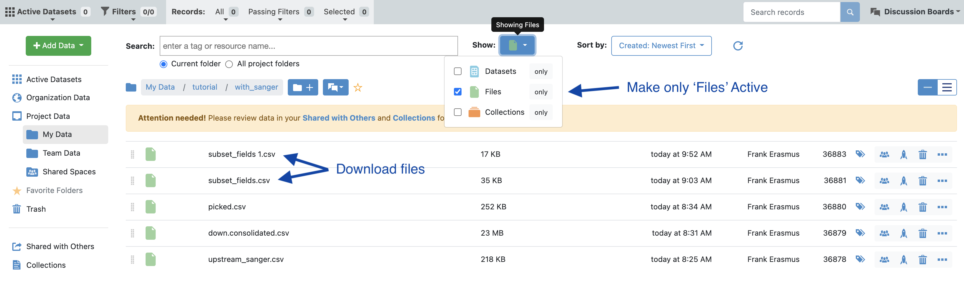
15. In data directory make only files active and download the csv files corresponding to the selected population.