Tutorial 5: NGS Pipeline with Automated Top Lead Selection (PacBio), Patient Library

Background

An antibody library from a convalescent patient exposed to wild-type SARS-CoV-2 was produced. To achieve this end, cDNA derived from reverse transcription using primers targeting the constant regions of the Ig(gamma) heavy chain as well as the constant regions of Ig(kappa) and Ig(lambda) light chains. Full-length VL and VH sequences were assembled using overlap PCR methodologies and cloned into Specifica vectors suitable for use in phage and yeast display. This patient-derived library was subject to selective pressure against the SARS-COV-2 antigen S1 antigen carried out under less stringent and more stringent conditions using high concentrations (aka early, e.g., 100nM) and low concentrations (aka late, e.g. 10nM) of antigen. One additional selection was carried out against a negatively sorted population (e.g., against populations against carrier Streptavidin populations only). DNA was isolated from both populations and each population was prepared by PCR amplification with the addition of in-line barcodes consisting of 8mer (DNA) sequences at the 5’ and 3’ ends to distinguish the 6 populations consisting of:

1) 2 x Kappa Light Chain populations (early and late)

2) 2 x Lambda Light Chain populations (early and late)

3) 1 Kappa Light Chain Negative Sort (late only)

A barcode table titled ‘patient_barcode.xls’ indicates how these samples were prepared. Amplified DNA products were pooled together in a single tube and shipped to a PacBio sequencing provider. The provider then shipped us back one PacBio file titled ‘patient_tutorial.fastq’. The PacBio file consists of set of sequences each of length ~800bp composed of variable light (VL) and variable heavy (VH) sequences in VL-linker-VH orientation.

For the purposes of this tutorial, each of the returned FASTQ files from PacBio/Illumina was reduced by taking a random output of 25,192 sequences for PacBio. These files are reduced with an anticipated full-length non-redundant diversity of ~2k.

The goal of the tutorial is to utilize a different dataset (e.g., patient library) that does not require any customized annotation file. Additionally we will employ other common clonotyping strategies (e.g. Hamming distance). We not only utilize the automated selection algorithm to select clones but will look into the Analyze tool to select populations from distinct scaffolds and clusters, with favorable characteristics that were not initially selected by our automated pipeline.

STEP 1 - Login to Orion, Set-Up Directory, Upload Files

1. If the sequencing provider provides FASTQ files that are compressed (e.g., ends with “.gz” or “.zip”), decompress with a standard decompressor so the file ends with .fastq. If any suffix is added to the end, make sure to modify these suffixes so they end in .fastq for all sequence files to be processed.

2. Log into the Orion interface with your email and password. Find the 3 required files under Organization Data as follows:

   A) Organization Data / OpenEye Data / Tutorial Data / AbXtract / patient_tutorial.fastq

   B) Organization Data / OpenEye Data / Tutorial Data / AbXtract / patient_barcode.xls

3. Create a general tutorial directory and tutorial 5 subdirectory under PROJECT DIRECTORY / TUTORIALS / TUTORIAL_5 (This is your BASE DIRECTORY and should be used for all outputs for this Tutorial 5 below).

STEP 2 - Select the ‘NGS Pipeline with Automated Lead Selection’ Floe

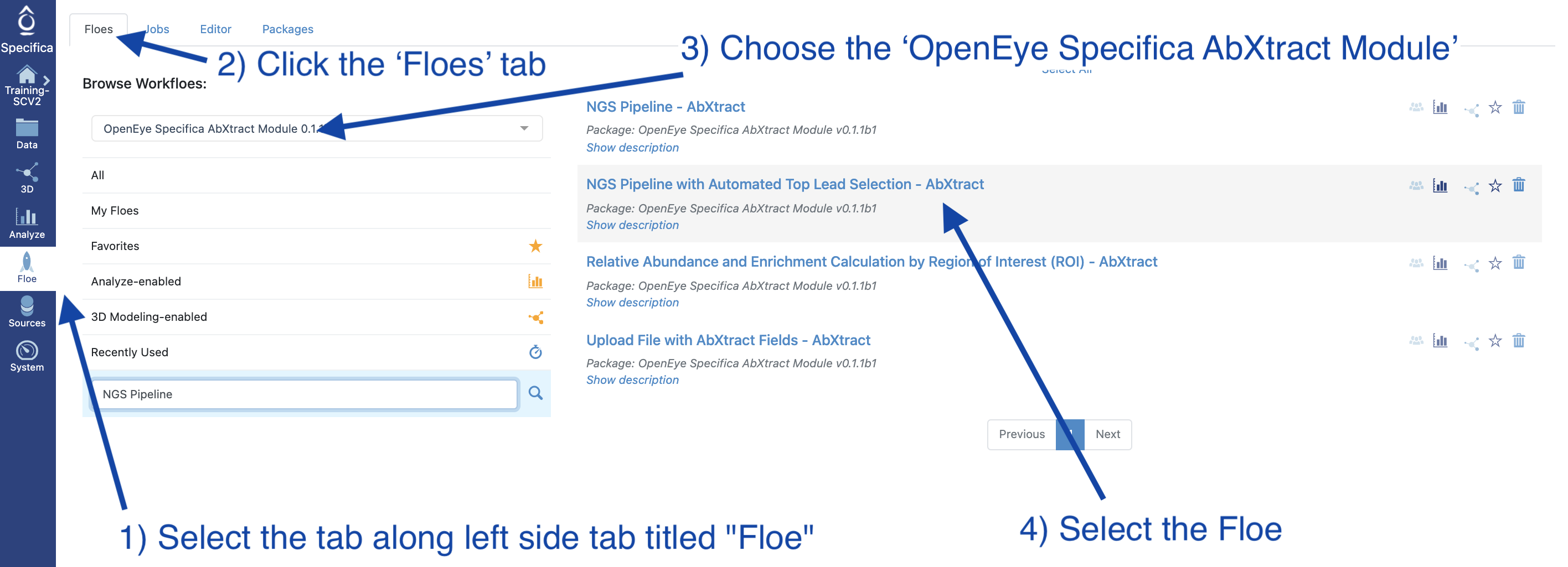
1. Select the tab along the left side tab titled ‘Floe’.

2. Click the ‘Floes’ tab.

3. Choose the ‘OpenEye Specifica AbXtract Module’.

4. Select the Floe ‘NGS Pipeline with Automated Top Lead Selection’.

STEP 3 - Prepare PacBio Run and Start Job

1. Make sure to specify (and remember) the directory output for all datasets and files.

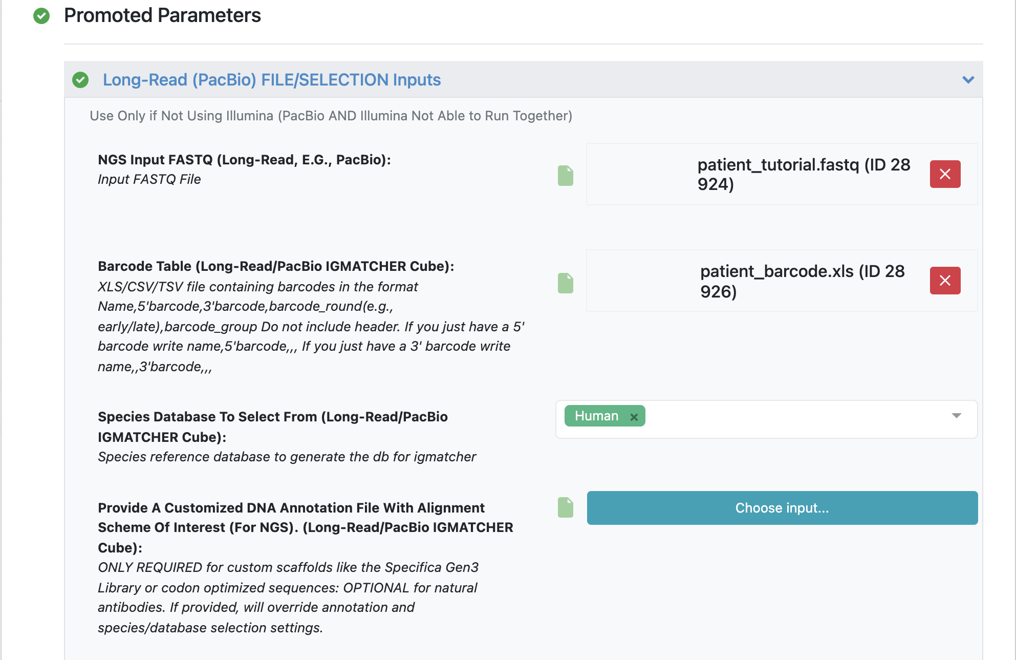
2. Load FASTQ file - ‘patient_tutorial.fastq’.

3. Load barcode XLSX file - ‘patient_barcode.xls’.

STEP 4 - Select Different Clonotyping Method

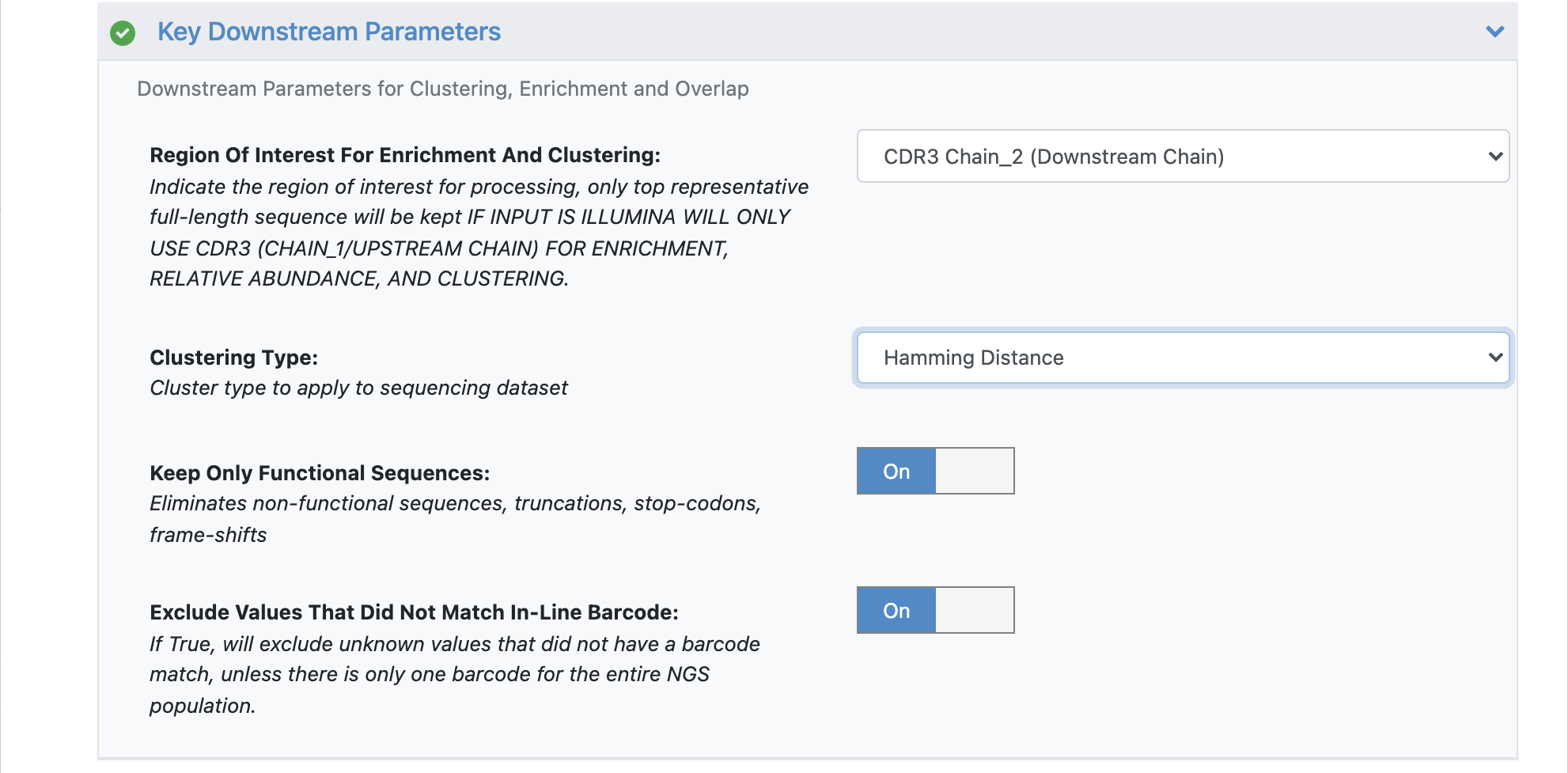
1. Under the promoted ‘Key Downstream Parameters’, click to expand.

2. Change the ‘Clustering Type’ to ‘Hamming Distance’.

3. In order to adjust the maximum Hamming distance (default = 2) we need to open the ‘Hidden Parameters’.

4. Turn the option ‘Show cube parameters’ to ‘Yes’.

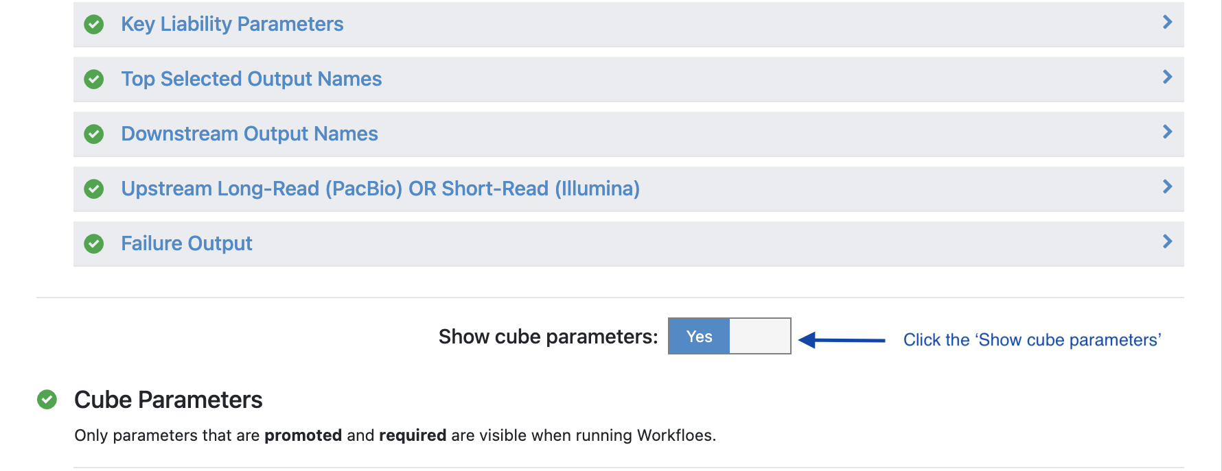
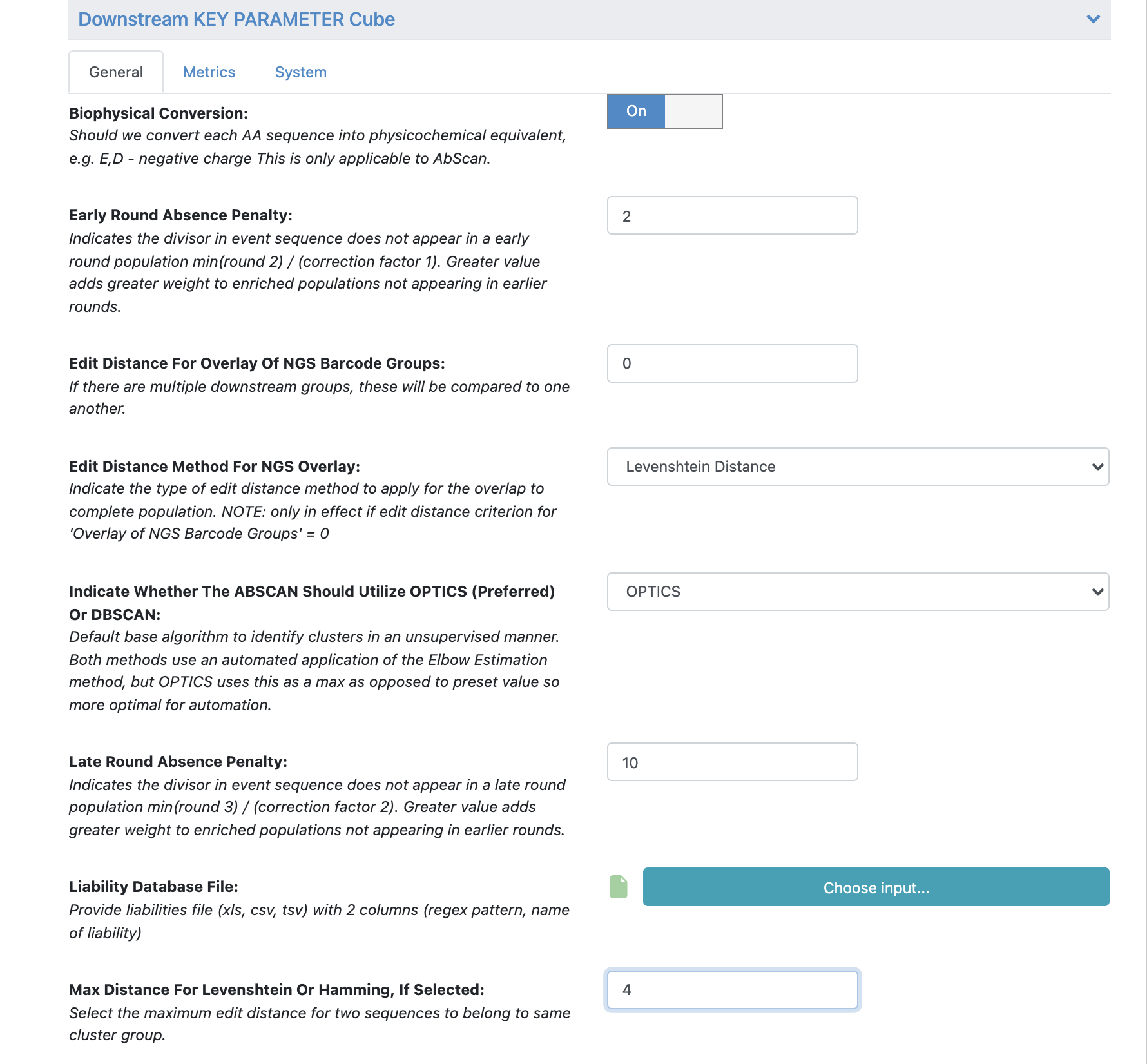
5. Under ‘Cube Parameters’ find the box titled ‘Downstream KEY PARAMETER Cube’. Click to expand.

6. Find the ‘Max Distance for Levenshtein or Hamming, If Selected’. Change this value from 2 to 4.

All the remaining parameters can be kept as the default values. Scroll through remaining “Promoted” parameters to understand these in greater detail.

See tutorial 2 automated selection options for more details.

7. Click ‘Start Job’.

STEP 5 - Identify both the Picked and the Downstream Population

1. Find the output directory specified above.

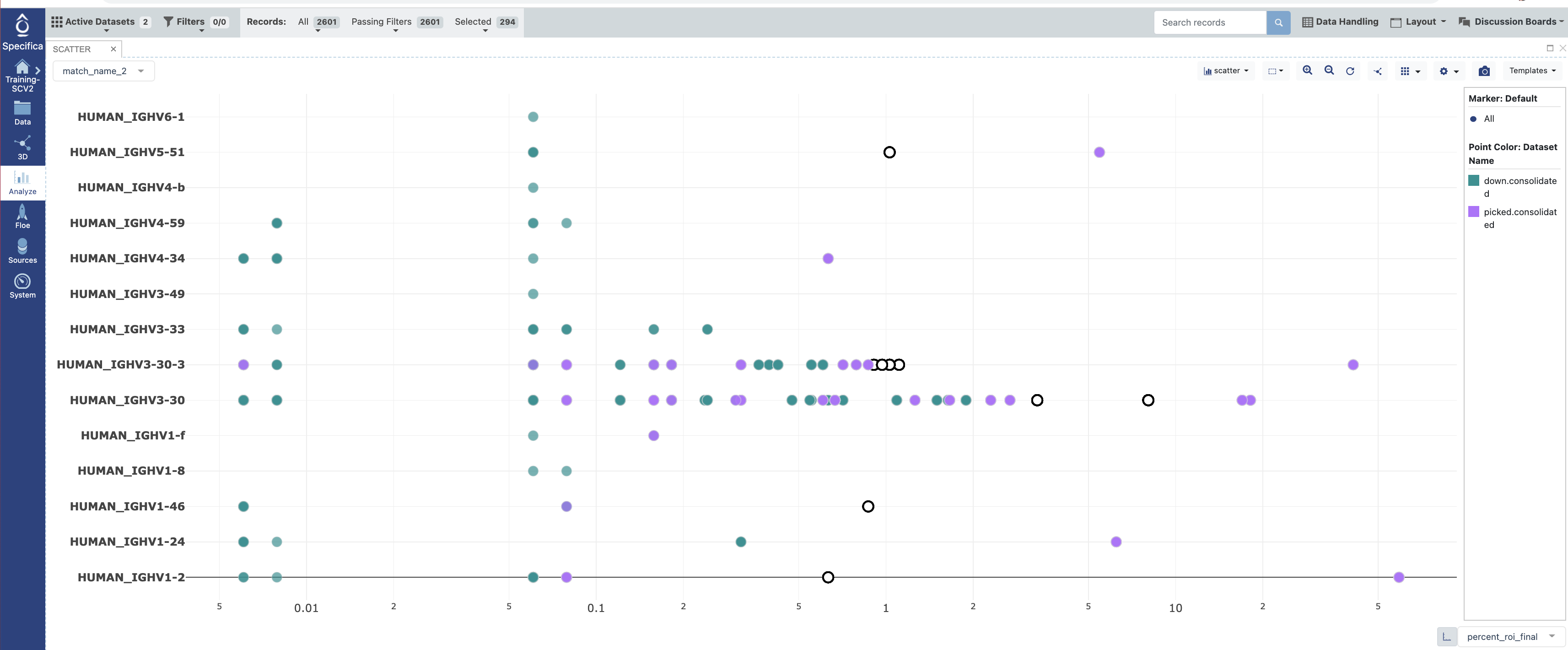
2. Identify the datasets labeled ‘picked.consolidated’ and ‘down.consolidated’ make both of these datasets active.

3. Open in the Analyze function and plot ‘percent_roi_final’ on the x-axis with the ‘match_name_2’ on the y-axis.

4. Under the settings for the plot color code the points by the “Dataset”.

5. Select populations found in the ‘down.consolidated’ dataset only, not the ‘picked.consolidated’.

6. Follow #12-14 under STEP 5 of Tutorial 3. We will ignore the well_id output as Sanger sequencing was not performed here.

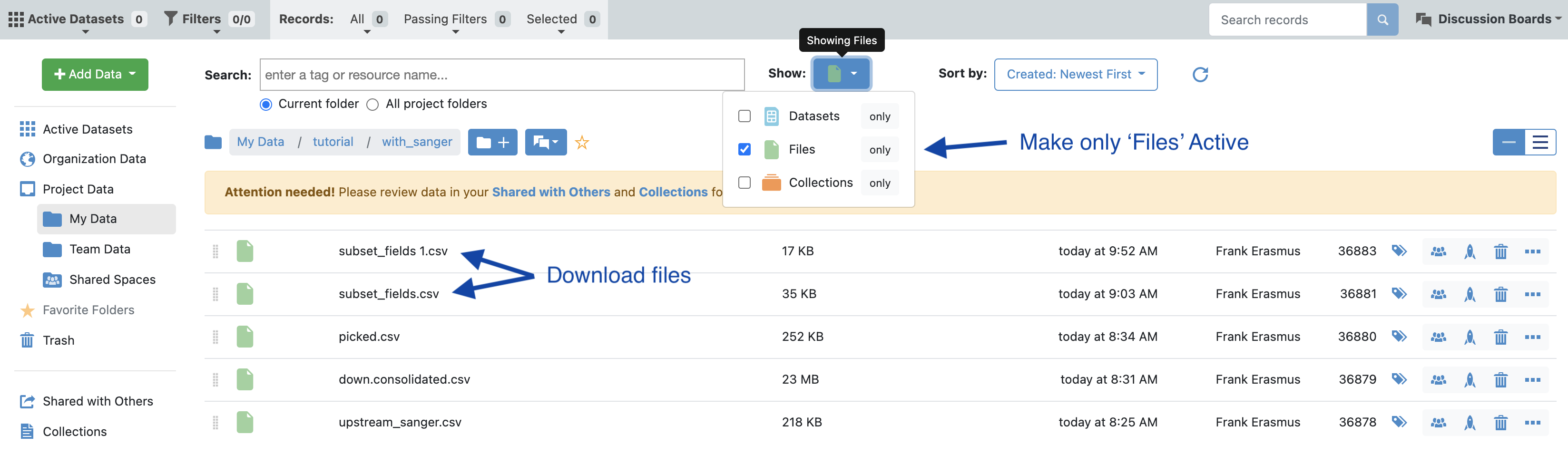
7. In the data directory, make files visible (see image) and download the csv files corresponding to the selected population. In this case we want the ‘subset_fields.csv’ which is derived from the additional clones selected in the Analyze tool as well as the ‘picked.csv’ which is the automated pipeline picked population.