How to Build Optimal Property-Predicting Graph Convolutional Neural Network Machine Learning Model by Tweaking Neural Network Architecture
This package helps chemists quickly explore chemical space, prioritize promising candidates, and gain deeper insights, accelerating the drug discovery pipeline. The user-friendly ML Build: Graph Convolution Model on Pregenerated Features for Small Molecules is designed to streamline drug discovery and materials science. We aim to simplify the process of building and using deep learning models for molecular property prediction.
This floe and the ML Predict: Graph Convolution Model Prediction Floe use Graph Convolutional Neural Network (GCNN) models for model building and property prediction. GCNNs can learn directly from the molecular graph using atom and bond features from OpenEye toolkits rather than features derived from the molecule (for example, fingerprints). GCNNs have an advantage over fingerprints in that there are no hash conflicts and there are fewer parameters for the model to learn. GCNNs are also not limited to interaction radii from complex structures, therefore building more generalizable models.
Key Features
Comprehensive Featurization: Uses all relevant OEChem features for detailed molecular insights.
Automated Architecture: Automatically sets the optimal Graph Convolutional Neural Network (GCNN) architecture based on your input data, saving you time and effort.
Actionable Reports: Provides a statistical Floe Report with guidance to prevent overfitting and easily train models.
Confident Predictions: Offers predictions with confidence intervals and an explainer feature for clear understanding.
Optimized Performance: Automatically chooses effective convolution layers and batch size for your specific task.
Scalable: Leverages PyTorch DDP to efficiently train on large datasets across multiple GPUs.
Preparing Your Data for GCNN Training
To build and predict the Graph Convolutional Model, refer to the Data Processing Floe tutorial. In this How-to Guide, we will give an intuition behind the different knobs you turn to build and predict models.
You will need to prepare your molecular data using the Data Processing of Small Molecule for ML Model Building Floe, (specifically, the Graph Feature Vector Generation parameter). This step creates a crucial collection of graph feature tensors, with each tensor representing a molecule in your dataset. This parameter builds graph feature tensors and outputs a collection with graph nodes and edge features that will be used as input for the GCNN model building floe.
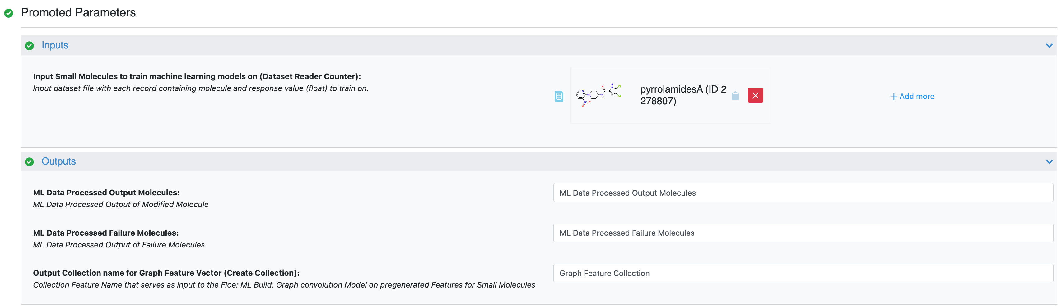
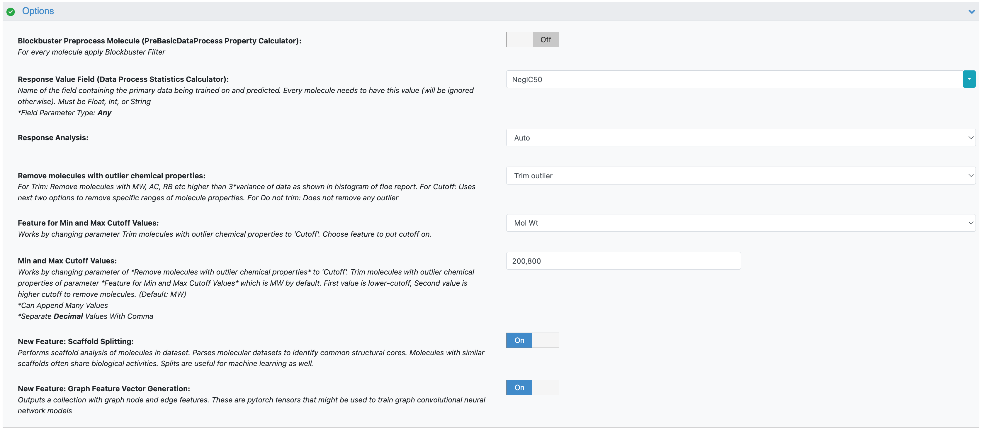
Figure 1. Parameters for the Data Processing of Small Molecule for ML Model Building Floe.
Think of this as the “featurization” step where your molecules are converted into a format (graph feature vectors) that the GCNN can understand.
Note
Two important aspects are implicitly determined by your data and previous choices in this floe:
Model Task: If you select the variable in the Response Value Field as an integer or string field, the floe will automatically configure a classification model. If you select a float field, it will build a regression model.
Test Data Handling: If you opted for a scaffold split during data validation in the Data Processing Floe, then that specific held-out test dataset will be preserved and used consistently. If you chose a random split, the builder floe will randomly select test data during each run. Please note that the Output Dataset (Prediction Writer) validation port will output validation data for scaffold splits only as we hold onto the scaffold validation records.
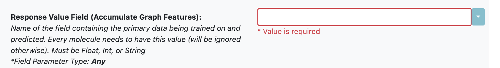
Figure 2. The parameter for the model task.
Figure 3. The parameter for test data handling.
Connecting Data for GCNN Builder
The output from the Data Processing of Small Molecule for ML Model Building Floe, specifically the collection generated under the Output Collection Name for ML Build: Graph Convolution, will serve as the input for your training and validation data for the ML Build: Graph Convolution Model on Pregenerated Features for Small Molecules Floe.
Data generation is separated from the model building floes to ensure modularity. This means you can reuse your preprocessed molecular data collection multiple times while you iterate and optimize your GCNN model’s architecture or training parameters.
Initial Setup and Model Automation
When you’re running this ML Build: Graph Convolution Model on Pregenerated Features for Small Molecules Floe for the first time, we highly recommend using all the default settings and automations in the Advanced Options parameter section.
One key automation is the Automatically Adjust Hidden Layer Size feature. This setting helps determine appropriate sizes for the graph convolution and fully connected layers within your GCNN, dynamically adjusting them based on the size of your input data.
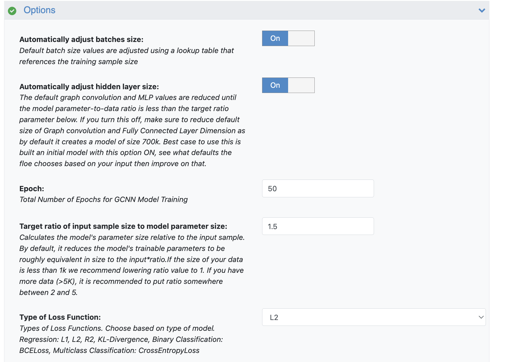
Figure 4. The Options parameters for the ML Build: Graph Convolution Model on Pregenerated Features for Small Molecules Floe.
It starts with a relatively large model (around 700K nodes) and then reduces the sizes of the hidden and MLP layers until the ratio of your ML Architecture’s Parameter Count to your training dataset size matches the value set in the Target Ratio of Input Sample Size to Model Parameter Size parameter.
As a general guideline:
If your dataset is small (less than 1,000 samples), consider lowering the Target Ratio of Input Sample Size to Model Parameter Size to 1.
For larger datasets (more than 5,000 samples), a ratio between 2 and 5 is generally recommended. This heuristic aims to strike a good balance between model complexity and the amount of data available for training.
Model Training, Evaluation, and Improvement
This floe leverages the PyTorch Geometric and PyTorch Elastic parameters to perform robust, multi-GPU, and batched cross-validation training, ensuring a high-quality model build.
Once the model build is complete, navigate to the Floe Report to evaluate its performance on the held-out test data.
Evaluation Metrics
Regression Models: You will see metrics such as Mean Absolute Error (MAE), Mean Squared Error (MSE), Pearson Correlation Coefficient, and R-squared (R2).
Classification Models: Metrics include Accuracy (Acc), Precision (Prec), Recall (Rec), and F1-score.
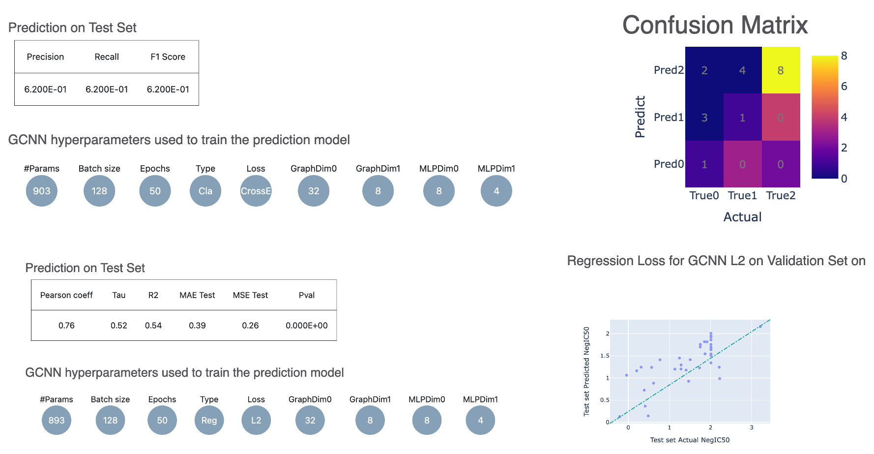
Figure 5. Evaluation metrics from the Floe Report for the ML Build: Graph Convolution Model on Pregenerated Features for Small Molecules Floe.
Interpreting Training Graphs and Next Steps
For background information about how to detect overfitting, see the guide about how to build an optimal property-predicting machine learning model.
The performance on test data, coupled with the training graphs (e.g., loss curves for training and validation), provides critical insights for model improvement.
Underfitting: If your training graphs show that both training and validation losses are high and not decreasing significantly, or if the model performs poorly on both training and test data, your model is likely underfitting. This suggests that the model is too simple to capture the underlying patterns in your data.
Action: To address underfitting, consider increasing the model’s capacity. You can do this by turning off the Automatically Adjust Hidden Layer Size automation and manually setting the model’s graph convolution and MLP layer sizes to values larger than the defaults chosen by the automation in this floe run. You can also re-enable the automation with a higher value for the Target Ratio of Input Sample Size to Model Parameter Size.
Overfitting: If the training loss continues to decrease significantly, but the validation loss starts to increase or plateau, your model is likely overfitting. This means the model has learned the training data too well, including noise, and is failing to generalize to new, unseen data.
Action: To combat overfitting, the best method is to find more input data. However, since that is not readily available, you may reduce the model’s complexity. Do the reverse of underfitting: manually set the graph convolution and MLP layer sizes to smaller values than the defaults, or re-enable the automation with a lower value for the Target Ratio of Input Sample Size to Model Parameter Size. Additionally, consider increasing regularization techniques like weight decay or adding dropout layers in the advanced section.
Generalization Issues (Beyond Over/Underfitting): If the model isn’t generalizing well even after adjusting the model size, consider changing the batch size. A different batch size can sometimes help the optimizer find a better solution or provide a smoother training landscape.
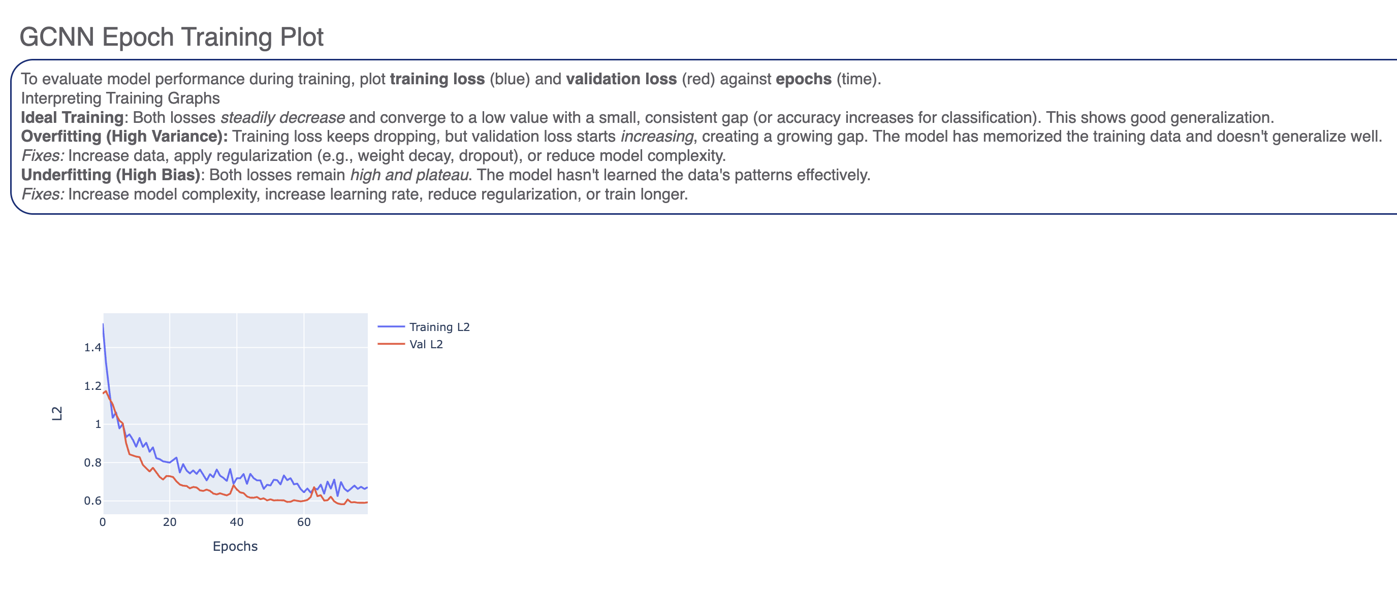
Figure 6. The GCNN epoch training plot.
Other Techniques to Evaluate and Improve Model Building
Data Quality and Quantity: Ensure your training data is high quality and representative of the chemical space you’re interested in. More diverse and accurate data often leads to better generalization.
Hyperparameter Tuning (Manual Exploration): Beyond just hidden layer sizes and batch size, you might explore other hyperparameters like learning rate or the number of epochs to make sure the training graphs converge. These can be found in the Advanced Options of the floe.
Error Analysis: Dive deeper into the specific predictions where the model performs poorly. For scaffold split, we emit the molecules and model predictions for them. Are there common structural motifs or property ranges where it struggles? This can guide further data collection or feature refinement.
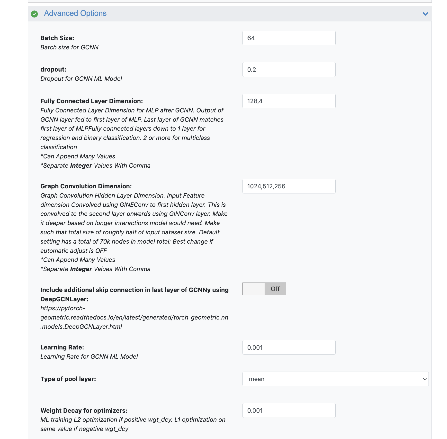
Figure 7. Parameters on the Job Form to use for hyperparameter tuning (by manual exploration).
Library Details of the Floe
This floe is built upon a robust foundation of cutting-edge deep learning and cheminformatics libraries, ensuring high performance, scalability, and chemical intelligence.
PyTorch: The core deep learning framework providing the tensor computation (similar to NumPy but with strong GPU acceleration) and the dynamic neural network capabilities that power our GCNNs.
PyTorch Geometric (PyG): An extension library for PyTorch specifically designed for building and training Graph Neural Networks (GNNs). It provides efficient tools, data structures, and implementations of various state-of-the-art GNN layers crucial for handling molecular graph data.
PyTorch Distributed Data Parallel (DDP): Utilized for scaling training across multiple GPUs. DDP efficiently distributes the model and data, synchronizing gradients across processes, which is essential for training large GCNNs on extensive datasets.
PyTorch Elastic: This library complements PyTorch DDP by providing fault tolerance and elasticity for distributed training. It helps manage the distributed training processes, enabling the floe to recover from failures and dynamically adjust to available resources. (Note: Many core features are now upstreamed into PyTorch’s torch.distributed.run.)