A Small Molecule Membrane Permeability Calculation

The OpenEye Permeability Floes are designed to be a user-friendly way to understand the mechanism of passive membrane permeability. The starting input is a small molecule (2D or 3D) on a record in a dataset, which is turned into a set of input systems (basis states) containing the molecule, a pre-equilibrated POPC membrane, and a layer of water to solvate the entire system. These basis states are used in weighted ensemble (WE) molecular dynamics (MD) simulations to predict the mechanism of passive permeation, as well as provide an estimate for the permeability coefficient.

A permeability estimate using this Floe package can be useful for the following reasons:

• Permeability liabilities can hinder progress of a promising lead candidate, and this tool will provide insight into the mechanistic process that prevents or permits acceptable permeation.

• Detailed knowledge and analysis of the permeation pathways provide insight into the bottleneck regions for a common lead series, which could help guide a medicinal chemist toward rational drug design for permeability.

The WE-MD method applies MD simulations and WE algorithm in an iterative fashion. In this tutorial, a small molecule (tacrine) will be prepared and run for a short simulation (10 iterations of 100 ps each in terms of molecular time). This short simulation will be analyzed using the analysis Floe, and the resulting data will be compared to a larger, pre-generated output dataset of the same molecule.

This tutorial uses the following Floes from the OpenEye Permeability Floes package:

• Permeability - Run Permeability Simulation;

• Permeability - Analyze Permeability Simulation;

• Permeability - Calculate Auxiliary Coordinates (Optional);

• Permeability - Continue Permeability Simulation (Optional).

Create a Tutorial Project

Note

If you have already created a tutorial project you can re-use the existing one.

Log into Orion and click the home button at the top of the blue ribbon on the left of the Orion Interface. Then click on the “Create New Project” button and in the pop up window enter Tutorial for the name of the project and click “Save”.

Orion home page

Launch a Permeability Simulation Job

In the Permeability - Run Permeability Simulation Floe, any 2D or 3D molecule can be used. However, for sampling concerns, users are encouraged to use molecules that fall within Lipinski’s Rule of Five. In this tutorial, a rigid small molecule acetylcholinesterase inhibitor, tacrine, will be used. The user will be instructed on how to prepare a molecule using the 2D sketcher, and will run the simulation for a short period (10 WE iterations).

The steps to prepare the dataset and run the permeability are detailed below.

Prepare Input Molecule

Note

If you have already created a dataset for use in the Permeability - Run Permeability Simulation Floe, you can choose to use it and skip this section.

1. An input dataset must either be select or generated on-the-fly. Here, we will generate tacrine on-the-fly using the 2D sketcher.

2. Click on the Input Dataset button (Choose Input…), and click on the 2D Sketcher tab.

3. Copy and paste the SMILES for tacrine into the 2D Sketcher: Nc1c2c(nc3ccccc13)CCCC2.

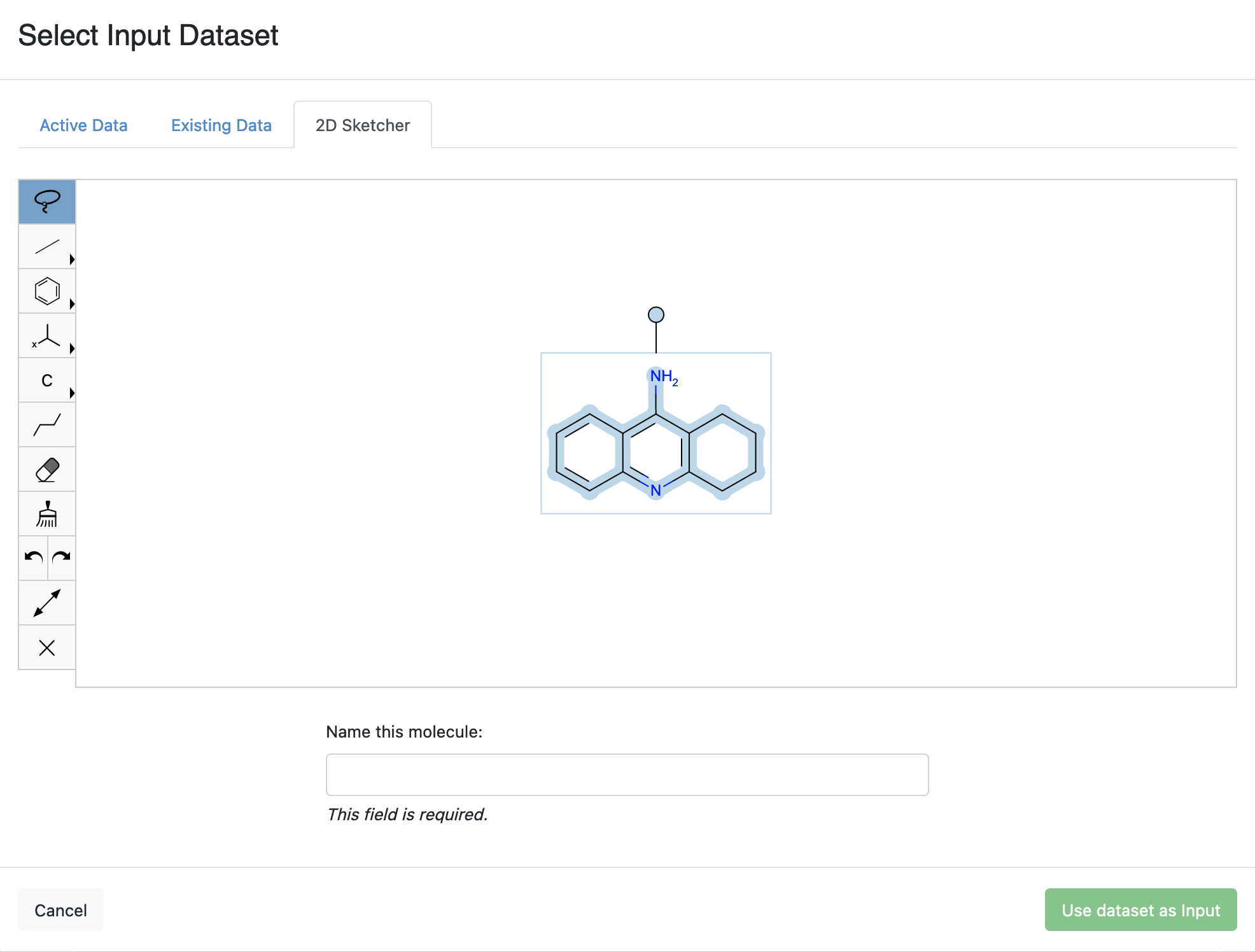
2D Molecule Sketcher

Set the molecule name to “Tacrine” in the “Name this Molecule” field, and then click the “Use dataset as input” button.

Warning

All the Permeability Floes can only run one molecule at a time, so if your dataset contains multiple records, only the last one will be taken as the input by the Floe.

Locate the Simulation Floe

1. Click on the “Floes” button in the left menu bar.

2. Click on the “Floes” tab.

3. Click “All Floes” under the “Filter Floes By” section on the left hand side to remove previous filters if there is any.

4. From the “Categories” on the left hand side, select Solution-based > Small Molecule Lead-opt > ADME & Tox > Permeability.

5. Find the Permeability - Run Permeability Simulation Floe from the results shown on the right hand side.

Note

Alternatively, you can locate the permeability Floes by typing “permeability” in the search bar. This is a convenient way to find floes that you don’t know their categories.

Click on the Floe and a Job Form will pop up. Specify the following parameter settings in the Job Form.

Modify Floe Parameters

Since an actual production permeability run (500 iterations) can be expensive, in this demo, we will run a short simulation of 10 iterations. Under the “Weighted Ensemble Parameters” section, change the number of iterations from 500 to 10.

Warning

If you leave the value at the default setting (500 iterations), this run may cost around $1800.

Note

For a real permeability job run, running 500 iterations is recommended for the simulation to converge.

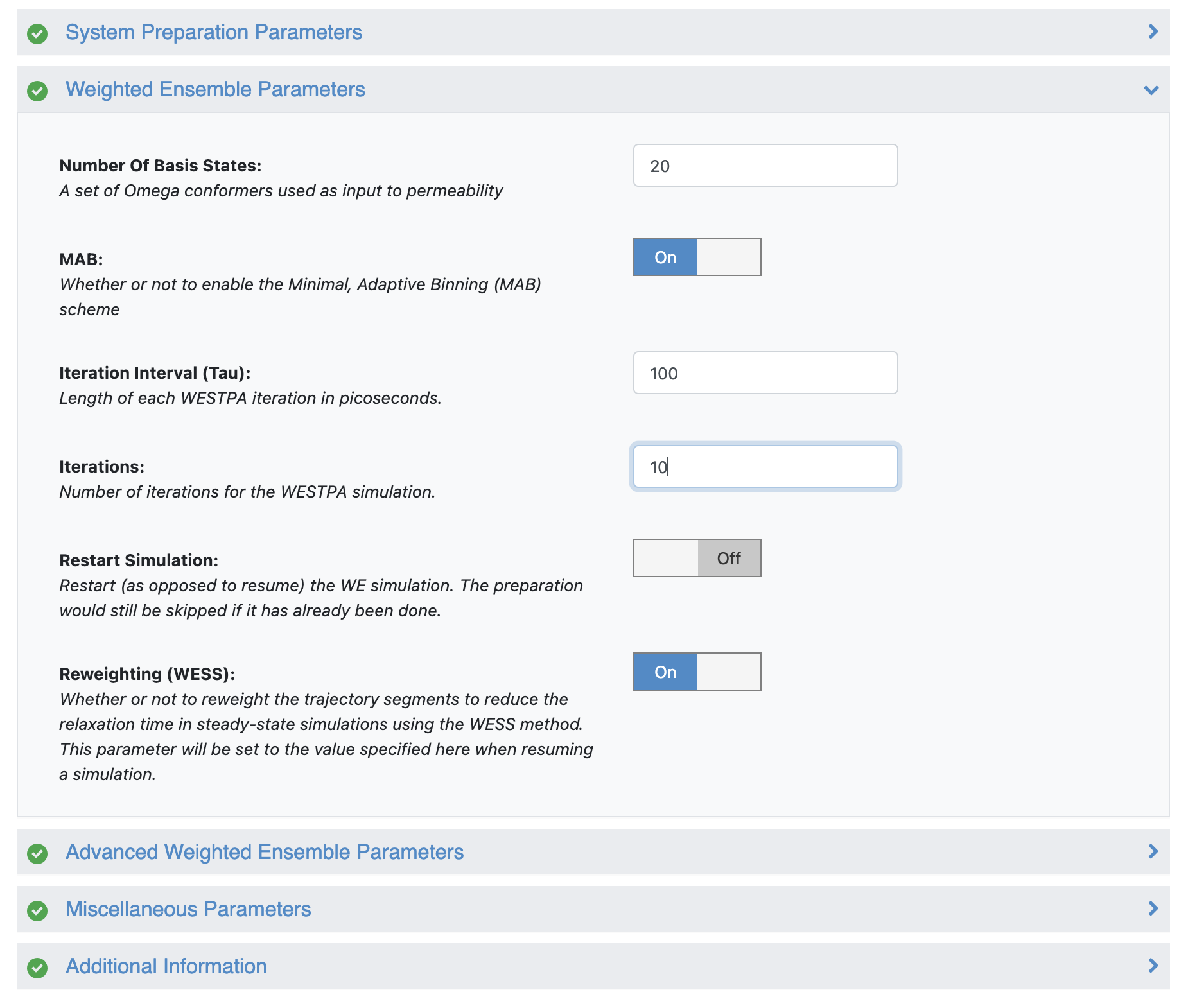
Set iteration number in the Job Form

Execute the Floe

Click the “Start Job” button to launch the floe. Wait for the Floe status to be complete before moving on to the next step in the tutorial (include system preparation, a set of 10 iterations will take approximately 1 hour).

Monitor the Floe Run (Optional)

While the permeability simulation is running (as indicated by the “Status” of the job in the “Jobs” tab of the “Floe” page), the progress of the simulation can be monitored by setting the output dataset as an “Active Dataset” and inspecting it in the “Analyze” page.

1. Open the running job page and locate the output dataset by clicking “Show in Project Data”;

2. In the “Data” page, add the output dataset to active data by clicking the “+” symbol before the dataset name;

3. Go to the “Analyze” page and inspect the records in the output dataset.

4. Find the columns named “Iteration Number” and “Maximum Iteration Number”.

Each iteration will output one record into the dataset. The records will be accumulated as the simulation progresses. The simulation finishes when “Iteration Number” matches “Maximum Iteration Number”, which was set up when launching the simulation job (see Modify Floe Parameters). So, if the last record in the output dataset has an iteration number that is smaller than the maximum iteration number, it means that the job is not yet finished.

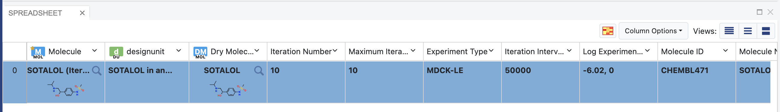
Iteration Number and Maximum Iteration Number of a finished job (10 iterations)

The dataset also contains information and statistics on the job for each iteration. You can also visualize these data during the course of the simulation using the SCATTER plot in the “Analyze” page. This can be achieved by setting the x-axis to Iteration Number and y-axis to another column, such as Segment Count, Wall Clock Time, or CPU Time.

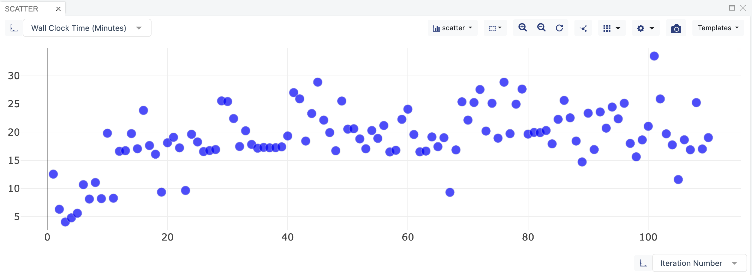
Wall Clock Time versus Iteration Number. The data points show how long it has run for each iteration.

Resume/Restart a Previous Job (Optional)

The simulation can stop unexpectedly due to various reasons, including but not limited to connection issues or system setup errors. In this case, the job will be marked as “Failed” in the “Jobs” tab and the output collection may have a size of zero. The Permeability - Run Permeability Simulation Floe is designed to save checkpoints such that all the data that has been generated will be preserved and the simulation can be resumed from the last checkpoint. When such an early termination occurs, it is recommended to resume the simulation using the Permeability - Continue Permeability Simulation (Optional) Floe with the procedure provided below to ensure safe analysis of the simulation at a later stage.

1. Locate the Permeability - Continue Permeability Simulation (Optional) Floe the same way as shown in the Locate the Simulation Floe section and click on the Floe to open the Job Form.

#. Click on the “Choose Input…” button for the Collection input, and the find and select the output collection from the previous job as the input.

1. Change the value for “Iterations” in “Weighted Ensemble Parameters” to 20.

2. Click the “Start Job” button to launch the Floe.

Then the simulation will be extended to a total of 20 iterations.

Note that a new output dataset will be created by the new job, but the trajectory data will be added to the original collection that was used as the input for this job.

Note

The Permeability - Continue Permeability Simulation (Optional) Floe can be used to extend a finished simulation for extra iterations as well using the same procedure.

When resuming a job, most of the parameters are immutable and their values will be kept the same as what was used in the initial simulation, except for the following:

• Iterations. The simulation will be resumed to run up to the specified total number of iterations. If the specified number is smaller than the current number of iterations, then the Floe will still run one iteration.

• Reweighting, Reweighting Period, and Reweighting Window Size. Since the reweighting procedure can be applied at any point of the simulation, the Floe allows the user to turn on/off the reweighting feature when resuming a job.

Perform a calculation using CPUs instead of GPUs (Optional)

In the case of a severe GPU shortage on an Orion stack, one may want to run the permeability calculation using CPUs only. While it is possible, it is not advised to run in this manner due to the quite steep increase in cost per compound. Despite this warning, below we will demonstrate how to run the permeability simulation using CPUs.

At the bottom of the Job Form of the Permeability - Run Permeability Simulation Floe, slide the bar across so that “Show cube parameters” is in the “Yes” position.

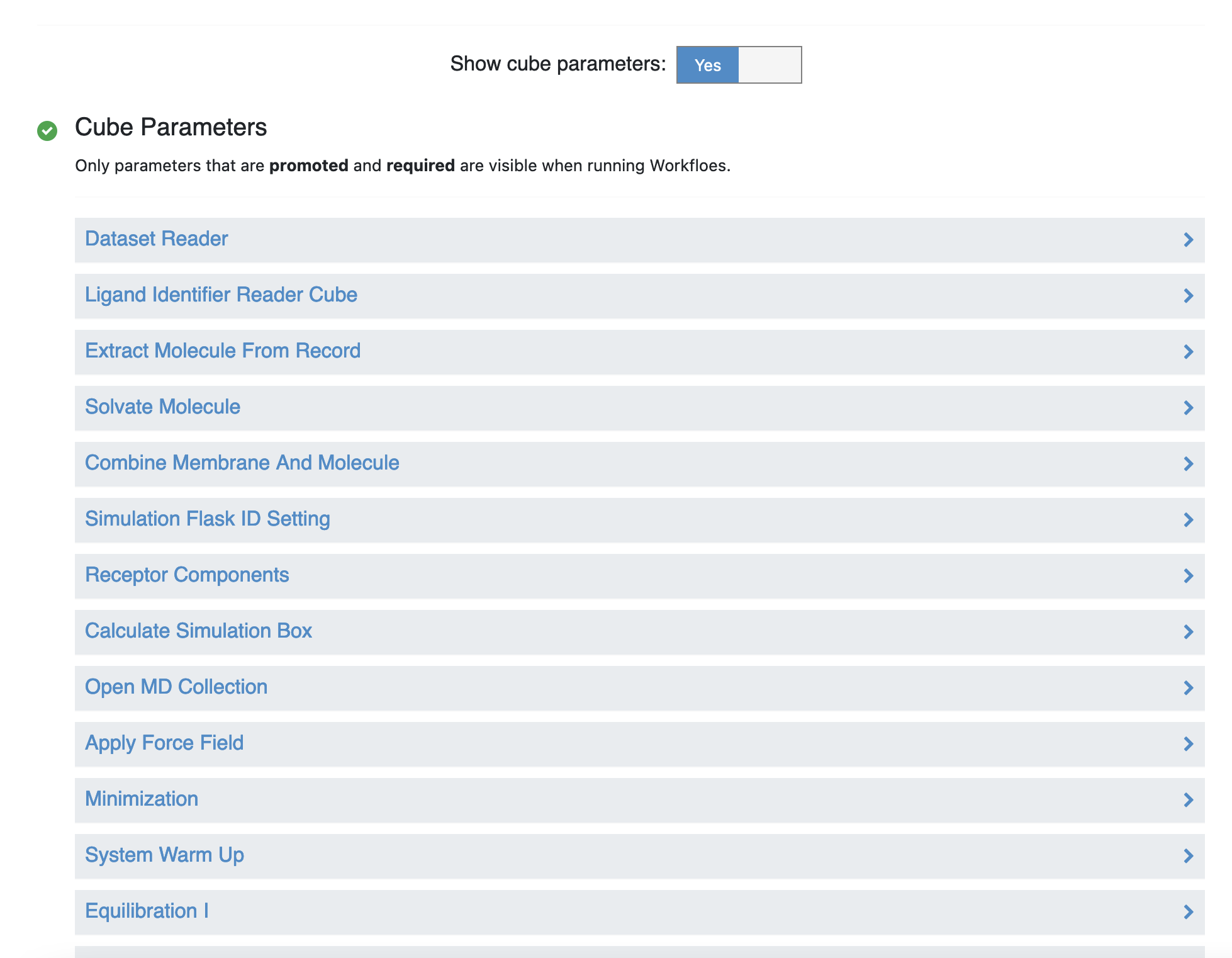
Under the Cube Parameters section, scroll down to the “Run WESTPA Segments (MD)” cube and click on the name to expand the cube parameters. Click on the “System” tab, and change the number of CPUs to 48, and change the number of GPUs to 0.

With these changes, the Permeability - Run Permeability Simulation Floe will now run with CPU instances.

Analyze the Permeability Simulation

This tutorial demonstrates how to perform basic analysis on the data generated by permeability simulation job. The set of steps needed to analyze any general output from a previously run will be presented here.

Warning

This tutorial only demonstrates how the Floe works. To obtain meaningful results, it is recommended to analyze a permeability run with 500 iterations.

Execute the Floe

1. Locate the Permeability - Analyze Permeability Simulation Floe the same way as shown in the Locate the Simulation Floe section and click on the Floe to open the Job Form.

2. In the Job Form, simply find and set the collection generated by the simulation job as the input collection.

3. Since no remaining parameters need to be set for analysis, simply click the “Start Job” button to launch the floe. Once the floe is complete, a floe report will be available.

Inspect the Results

Once the Permeability - Analyze Permeability Simulation Floe completes, it is best to visually inspect the results to assess the quality of the calculation. Here, we will discuss two important plots that are automatically generated to help the user inspect the quality of the results.

In the Permeability - Analyze Permeability Simulation Floe Report, a plot of the time evolution of the permeability estimate will be presented. An example from tacrine is presented below:

Here in this plot, one can see the permeability evolution as a function of the WE iteration number. Initially, the permeability estimate is 0 since there is no crossing events. This is due to the fact that without crossing events, no weight can make it to the target state in the acceptor water compartment on the opposite side of the membrane, which means the rate constant is 0 therefore the permeability is also 0.

Each time a crossing event occurs, more instantaneous weight is averaged into the rate constant and the permeability estimate “jumps” a small amount. A slow decrease in the permeability estimate could indicate that no new crossing events have been simulated, and the system lacks strong convergence.

Note

To go from iteration number to molecular time, simply multiply the amount of time simulated per-segment times the number of iterations. For instance, if each MD segment requires 100 ps, and there are 500 iterations total, then the total “molecular time” simulated would be 50 ns.

To gain a better sense of what exactly is happening inside the permeability simulations, one should also visually inspect the plot of the successful crossing events. An example from the same tacrine dataset is given below:

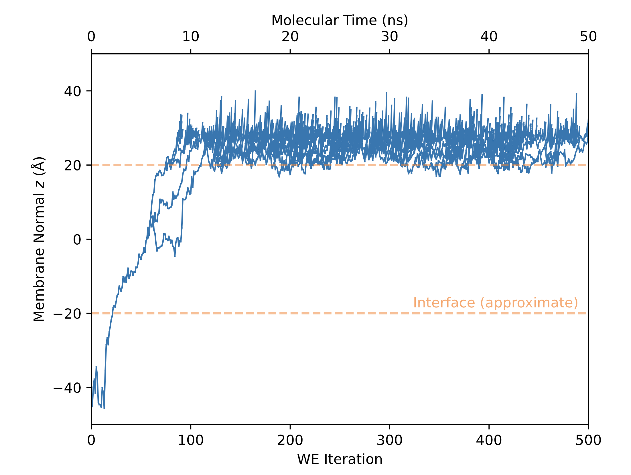
In this plot, the z-position of the successful crossing events are shown as a function of time. Here, roughly at iteration number 20, a single walker enters the membrane. At about iteration 50, the single walker splits into 3 separate walkers, where each separate walker attempts to exit the membrane through the opposing membrane leaflet. After about 100 iterations, all walkers are on the other side of the membrane attempting to escape to the acceptor aqueous phase.

Note

A small number of non-independent crossing events may lead to a permeability prediction that lacks statistical convergence. In such a case, multiple permeability simulations may be required.

What Does Bad Permeability Data Look like?

With any algorithm, it is important to know when you can, and more importantly when you cannot, trust your data. Here, we will show an example of a bad permeability result, and potential steps to correct the issue. For this section, it is assumed that you have already run the Permeability - Analyze Permeability Simulation Floe.

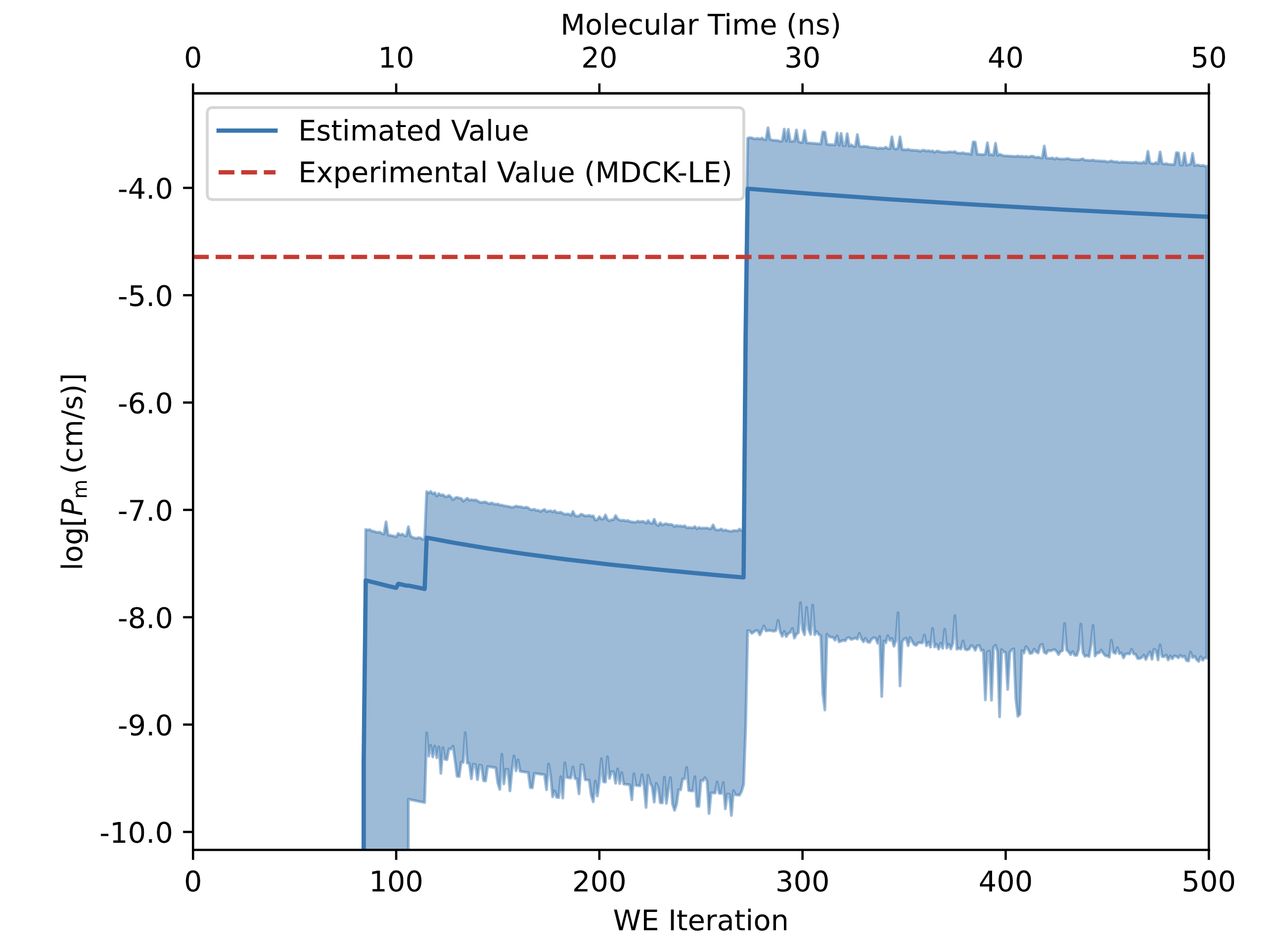
Below is an example of “bad data” that was generated with the Permeability Floe, and analyzed with the Permeability - Analyze Permeability Simulation Floe. First, take note of the permeability evolution plot:

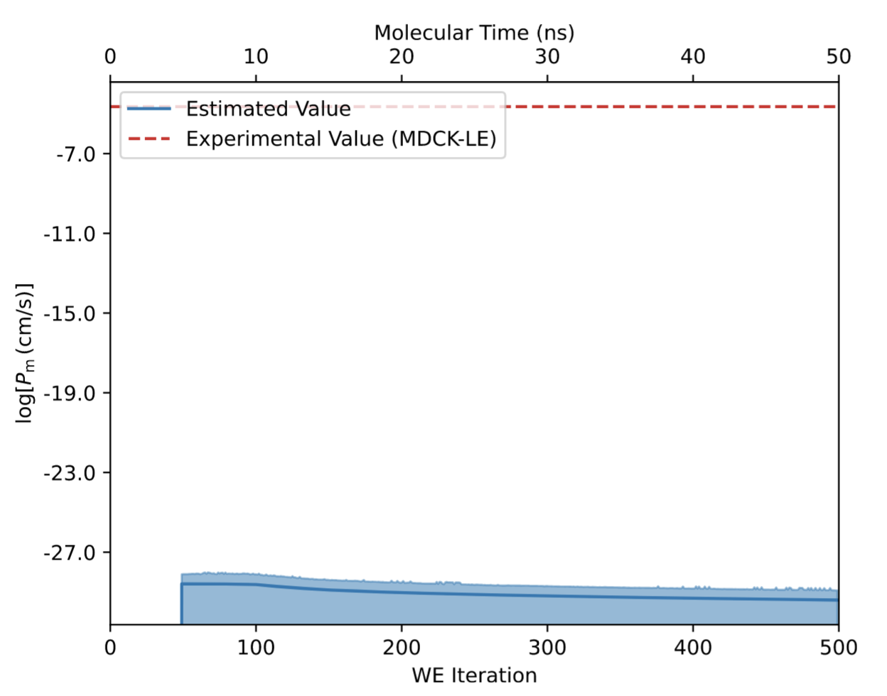
Here, one should observe the very low permeability value (~10 ^-30 cm/s) at the end of 500 WE iterations compared to the much more reasonable MDCK-LE experiment (10 ^-4.6 cm/s).

In order to understand the source of the erroneous prediction, it can be useful to look at the plot of the “successful” crossings. Below we provide the corresponding plot of “successful” crossing events for the unsuccessful simulation.

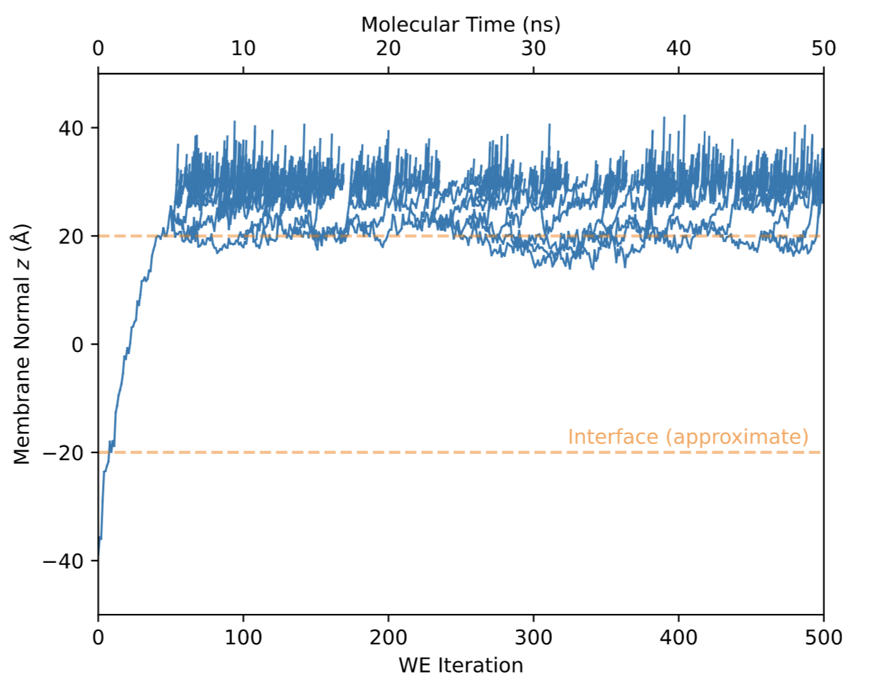
In this plot, one may notice only a single crossing event takes place during 50ns of molecular time. This crossing event occurs at roughly WE iteration 50, even before the first splitting can occur inside the membrane. This is a clear indicator that only one independent trajectory crossed the membrane, which is far too few for an accurate estimate of permeation kinetics.

Here are the following steps one might take to mitigate such an issue:

1. Continue the simulation for more WE iterations. It might be possible that an additional 10% of molecular time could provide enough sampling to produce another membrane crossing event.

2. Restart the permeability simulation from scratch. It may be that your particular system became kinetically or thermodynamically trapped in a state that it cannot escape, so a fresh restart could help this situation.

3. Is your molecule charged? If it is possible your molecule can have multiple charged states, check that a charged molecule was not inadvertently simulated. A charged molecule will likely have a low permeability value.

4. If you have large, highly flexible molecule, it is possible that a separate progress coordinate may be needed to improve conformational sampling. Please email support@eyesopen.com to discuss methods to facilitate this type of sampling within your permeability simulation.

Calculate the Auxiliary Coordinates

The main progress coordinate, that is the position of the molecule relative to the center of the membrane along the lipid bilayer normal (z), is calculated during the simulation. Additional coordinates of the system can be calculated using the Permeability - Calculate Auxiliary Coordinates (Optional) Floe. These additional coordinates are called auxiliary coordinates. Currently, 11 auxiliary coordinates can be calculated using the Floe:

• Cosine of the angle to \(\hat{z}\): the cosine of the angle of the molecule relative to the lipid bilayer normal, which is defined through the vector product of the unit electric dipole moment of the drug molecule and bilayer normal.

• No. of hydrophobic contacts: the number of hydrophobic contacts, which is defined to be the number of aliphatic atoms of the lipid tails within the 10 Å distance of any hydrophobic atoms of the drug molecule.

• No. of H-bonds to membrane: the number of hydrogen bonds between the drug molecule and the membrane, which is identified using the Baker-Hubbard definition.

• End-to-end distance (Å): the end-to-end distance of the drug molecule in Angstrom. The distance is defined as the maximum distance among all pairs of atoms in three dimensions.

• Hydration number: the number of water molecules within the first solvation shell (3Å) of the drug molecule.

• No. of H-bonds to water: the number of hydrogen bonds formed between the drug molecule and the water molecules.

• No. of H-bonds to water (acceptor): the number of hydrogen bonds formed between the drug molecule and the waters when the drug molecule is the acceptor.

• No. of H-bonds to water (donor): the number of hydrogen bonds formed between the drug molecule and the waters when the drug molecule is the donor.

• Desolvation penalty \(\Delta G`\) (kcal/mol): the desolvation penalty of the drug molecule calculated by OEZAP Toolkit. The desolvation penalty is calculated as the transfer energy of the molecule from a high dielectric (\(\epsilon=80\)) to a low dielectric (\(\epsilon=2\)) environment while the molecule maintains the same conformation. The penalty is composed of two main terms: solvation energy and surface area. For more information, see The Way of Zap.

• Solvation Energy (kcal/mol): the solvation energy calculated using Poisson Boltzmann.

• Surface area (\(Å^2\)): the surface area of the drug molecule in square Angstrom.

Execute the Floe

1. Locate the Permeability - Calculate Auxiliary Coordinates (Optional) Floe the same way as shown in the Locate the Simulation Floe section and click on the Floe to open the Job Form.

2. Set the collection generated by the Permeability - Run Permeability Simulation Floe as the input.

3. Click the “Start Job” button to launch the Floe.

Once the job is complete, the results will be presented in the Floe Report in the form of 2D probability distributions, where the main progress coordinate is the y-axis and each of the 11 auxiliary coordinates is the x-axis, respectively. A black line will overlay each 2D distribution, indicating the top weighted trajectory. These plots allow you to analyze the movement of the drug molecule through the membrane and observe specific chemical and physical changes it undergoes.

By default, these probability distributions are symmetrized along z to account for the symmetry of the membrane system. However, the original, unsymmetrized versions are also provided by unchecking the “Symmetrize” box at the bottom of the plots (it may take a while for the plots to update).