Dynamic Probe Analysis

Quick floe search term: CPD B1-C2

This floe can only be run with a protein sampling output generated from a water–xenon mixed–solvent simulation. This method detects pockets by finding sites that show cooperative changes in probe (xenon) binding.

Tip

This floe typically takes 10–12 hours to run and costs approximately $60.

Search and Run the Floe in Orion

Locate the Floe in Orion

Navigate to the Floe page using the blue navigation bar.

On the Floe page, click on the Floes Tab, where you will find a list of the available floes and packages.

Under the Category Floe Filters on the left, click on the caret next to the Packages filter to expand the list of packages and click on the OpenEye Cryptic Pocket Detection Floes package. This will ensure that the floes listed in the middle of the page are from this package.

From this list, click on the Dynamic Probe Binding Analysis Floe, and then click the “Launch Floe” button to launch the Job Form as shown in Figure 1.

Provide Input Files and Parameters to Run the Floe

• Output path:

  Select the destination for your output data by specifying the Output path.

• Input Data:

  You will need to provide a Protein Sampling Data collection generated by the Run a Weighted Ensemble MD Simulation Floe as an input.

• Output Data:

  You can customize the output dataset and collection names here.

• Cryptic Pocket Analysis Advanced Settings:

  Functionally important residues, such as active site residues or a known disease mutation, can be provided as input for the Important Residues parameter. These residues will be displayed along with cryptic pocket residues in the cryptic pocket analysis Floe Report. See the Dynamic Probe Binding Analysis Floe for additional details.

• Selection Range For Trajectories:

  Start Iteration: This parameter and End Iteration define the range of iterations to include in cryptic pocket analysis from the weighted ensemble simulations. The default setting includes all iterations starting from 1. By setting a number greater than 1 for Start Iteration, initial iterations can be excluded from the analysis. We do not recommend excluding initial iterations from the analysis.

  End Iteration: If left unspecified, the entire simulation dataset is analyzed. You can select a number lower than the total number of iterations for which your weighted ensemble MD simulation was run.

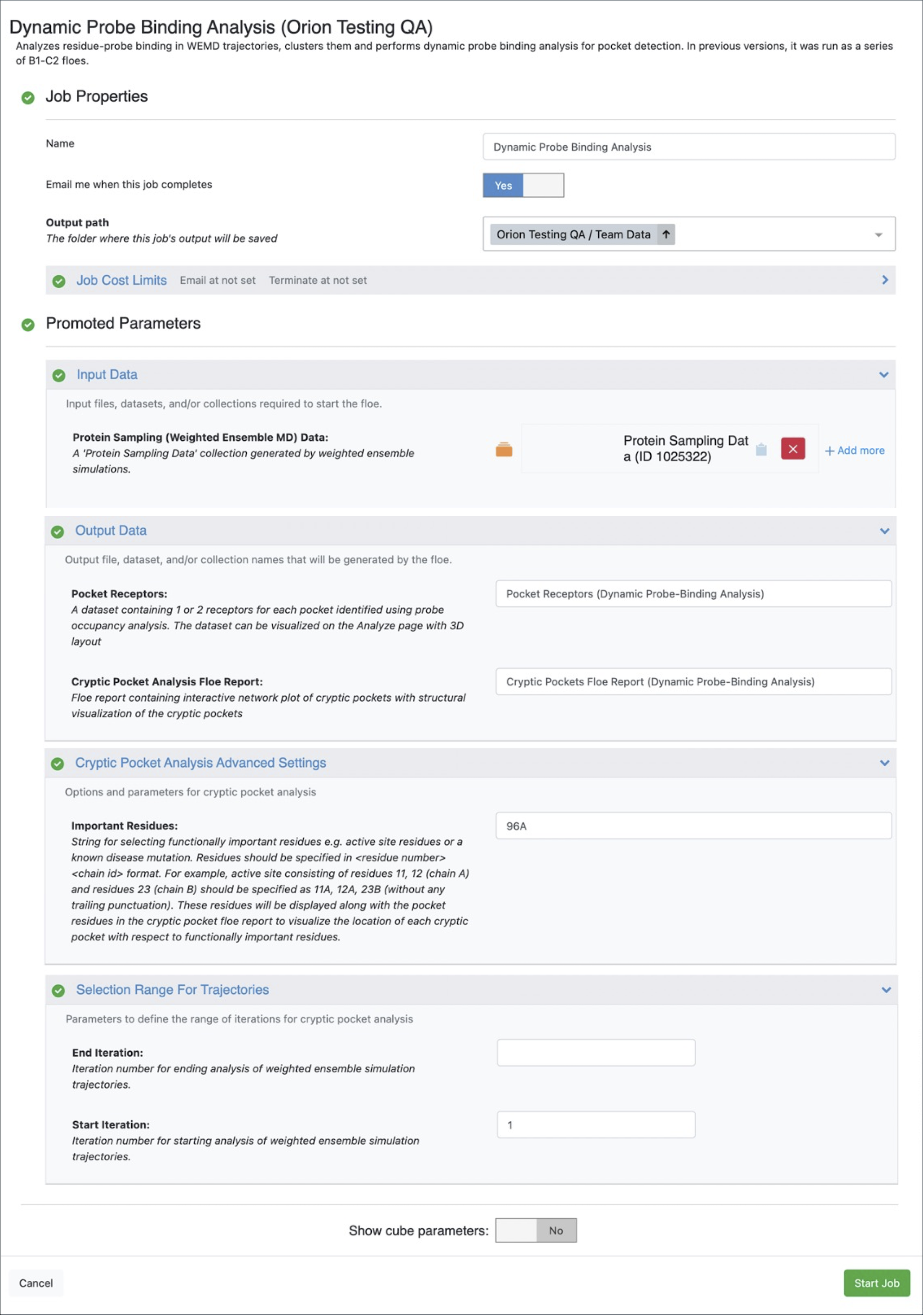
Figure 1. Job Form for the Dynamic Probe Analysis Floe.

Click on the green “Start Job” button.

Visualize Cryptic Pocket Analysis Report and Pocket Receptors

Cryptic Pockets Floe Report (Dynamic Probe Binding Analysis)

1. Access the Floe Report.

   When the job is complete, the output Cryptic Pockets Floe Report (Dynamic Probe Binding Analysis) should be inspected for visualization of cryptic pockets. To reach the Floe Report, navigate to the Jobs Tab on the Floe page and then click on the job that you want to inspect. Under Reports, click on the Cryptic Pockets Floe Report (Dynamic Probe Binding Analysis). This will redirect you to a report containing an interactive network plot of pockets detected as sites that undergo cooperative changes in the probe (xenon) occupancy.

2. Visualize the interactive network plot.

   Each node in the interactive network plot represents a pocket. The edge connecting two pockets corresponds to the inverse of the center-of-mass distance between those pockets. Node size corresponds to average intrapocket cooperativity in probe occupancy. The range of node colors corresponds to the number of pocket residues. By clicking on a node, a visualization of a representative protein configuration appears with the pocket-forming residues highlighted by a blue surface. If Important Residues input is provided by the user, those residues will be highlighted by a pink surface. You can visualize the residue side chains by clicking the “Show Residues” button at the lower-left corner of the page. Alternatively, clicking on an individual residue atom will show the label for that atom. Hovering over a node or the middle of an edge in the network plot will display the metadata associated with it.

3. Download ranked pockets data.

   You can download the ranked pockets metadata by clicking on the “RankedPockets.json” link at the bottom of the page. This file lists ranked pockets, their residue composition, and average intrapocket cooperativity in probe occupancy.

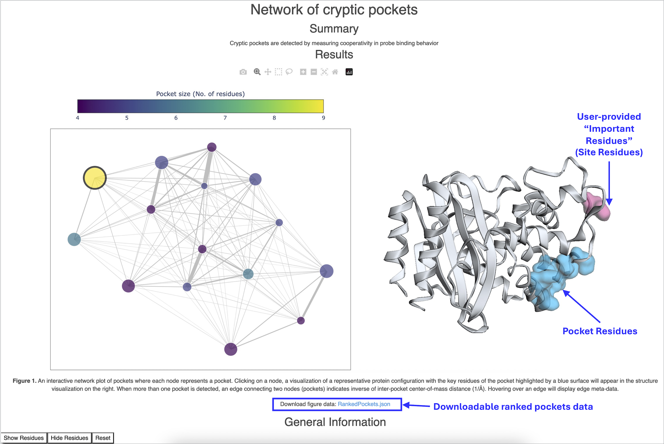
Figure 2. Interactive Network Plot.

Pocket Receptors (Dynamic Probe Binding Analysis) Dataset

1. Access the pocket receptors dataset.

   After the job is complete, you can get to the dataset (in this case, the dataset Pocket Receptors (Dynamic Probe Binding Analysis)) by clicking on the job. Navigate to the Jobs Tab on the Floe page. Click on the job that you want to inspect. Click on the “View in Project Data” button next to ‘Results.’ This will redirect you to the Data page and show only the outputs associated with the job. Next to the dataset (default name: Pocket Receptors (Dynamic Probe Binding Analysis)), click on the circle with a + sign to activate the dataset. It will change to a green circle with a checkmark and will allow you to view the dataset in the Analyze page and the 3D Modeling page.

2. Visualize pocket receptors dataset in the Analyze page.

   Using the navigation bar, go to the Analyze page. Make sure that your Active Dataset is set to your Pocket Receptors (Dynamic Probe Binding Analysis) dataset. On the scatter plot on the Analyze page, choose the Receptor Volume for the y-axis and Pocket Rank for the x-axis. Also click on the ‘Layouts’ drop-down in the Active Data Bar and select the Analyze with 3D option to visualize a design unit with a pocket receptor. This shows a depiction of the protein structures of the representative conformations with a receptor corresponding to a selected pocket and receptor volume.

   1. The Pocket Rank column in the Spreadsheet shows the pocket rank determined by the intra-pocket cooperativity in probe occupancy. The pocket rank 0 has the highest intrapocket cooperativity.

   2. The Receptor Volume column in the Spreadsheet shows the receptor volume for a pocket in a representative conformation selected from the cluster center conformations generated during cryptic pocket analysis. A representative conformation is selected for each pocket (dynamic probe binding site). This conformations has the highest receptor volume within the range 100 to 1500 ų.

   3. The Reference Receptor Volume column in the Spreadsheet shows the receptor volume for a pocket in the equilibrated structure used to start the weighted ensemble MD simulation. Comparison with the Receptor Volume provides an indication of the pocket opening and closing during simulation.

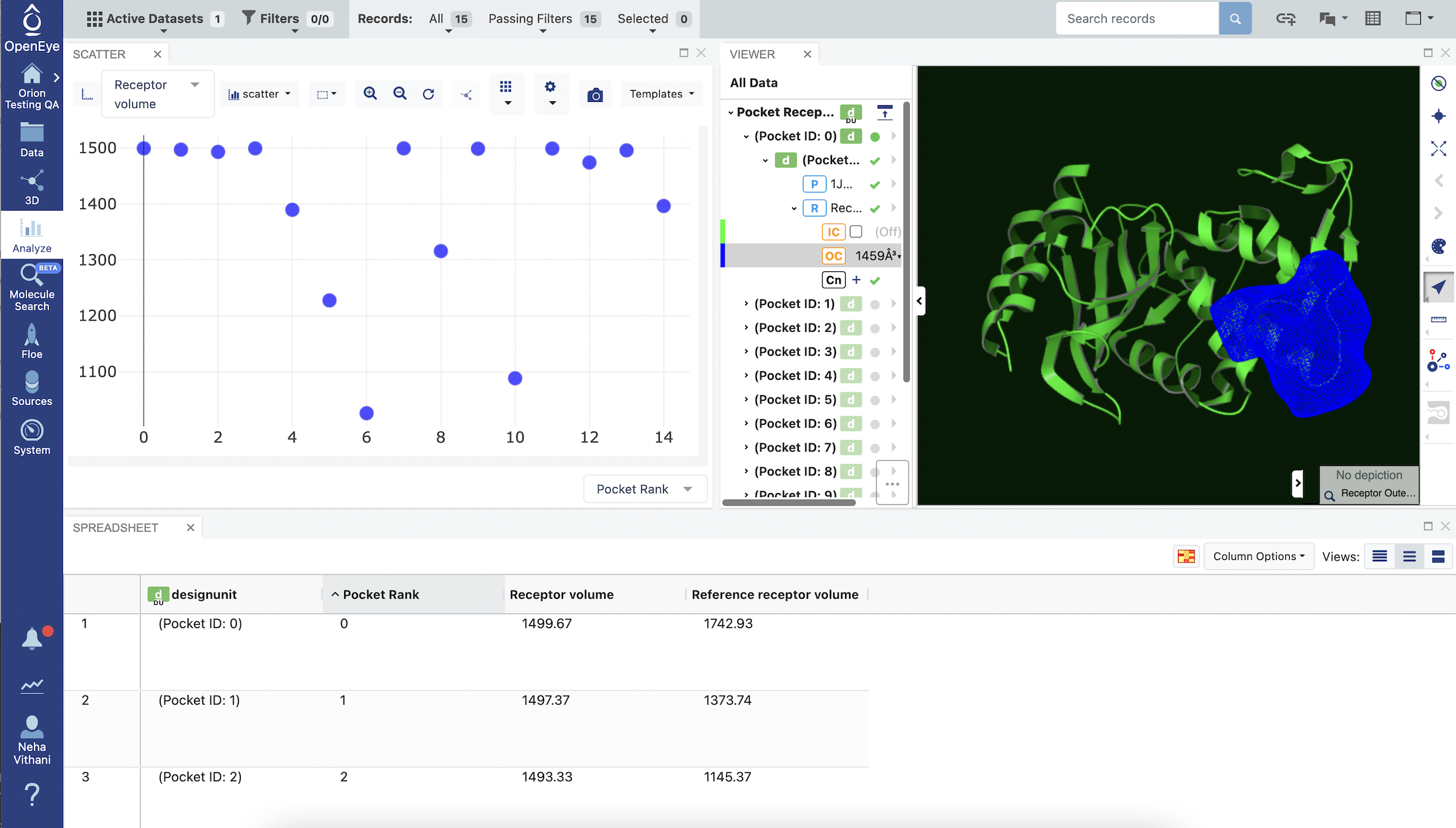
Figure 3. Pocket Receptors (Dynamic Probe Binding Analysis).

3. Sort and Select Pocket Receptors:

   Clicking on the Pocket Rank column in the Spreadsheet sorts the pockets by their rank, in either ascending or descending order.

   1. After sorting the structures by rank in the Spreadsheet, click on a row with the Pocket Rank and Receptor Volume values of choice. This will display the protein structure in the Viewer panel corresponding to the selected row.

   2. Under All Data, click on the small caret next to the corresponding design unit to display all components present in this design unit.

   3. Click on Receptor, Inner Contour (IC), and Outer Contour (OC) to visualize the receptor. The receptor will appear in blue-colored mesh. After visualizing different design units and their receptors, you can select an appropriate design unit for Gigadock or SiteHopper analysis.

Failure Report

Your job might fail and generate a Failure Report. Open the Failure Report to see the instructions. The analysis can fail for multiple reasons.

• The cryptic pocket detection method you chose failed to detect a pocket. It is possible that one or all of our cryptic pocket detection methods fail to detect the pockets. All three methods use different approaches and define “cryptic pockets” in a different manner. For example, the Dynamic Probe Binding Analysis Floe will fail if no sites with cooperative changes in probe occupancy were identified.

• No significant conformational changes associated with cryptic pocket formation were observed during the simulation. This could happen because of insufficient sampling or when the normal modes used as progress coordinates could not efficiently sample pocket formation. You may consider extending your weighted ensemble MD simulation using the Continue a Weighted Ensemble MD Simulation Floe and rerun the cryptic pocket analysis with the extended protein sampling. Alternatively, you can perform another weighted ensemble MD simulation using a different set of normal modes as progress coordinates with high variance in the region of interest in the target protein.

• It is also possible that your target protein is highly inflexible; therefore, it doesn’t show conformational changes that can potentially reveal a cryptic pocket.