Theory: The Application of Neural Networks to OpenEye Model Building
Theory: The Application of Neural Networks to OpenEye Model Building
When discussing the details of the floes contained in this package, it’s important to explain some rudimentary
information about machine learning and neural networks. The extension of the basics will also be extended to outline
how neural networks apply to OpenEye tools.
Dr. Robert Hecht-Nielsen, the inventor of one of the first neurocomputers, defined an Artificial Neural Network as:
“ ..a computing system made up of a number of simple, highly interconnected processing elements, which process information
by their dynamic state response to external inputs.”
Simply put, a neural network is a set of interconnected nodes or mathematical modules (just like neurons in our brain)
that collectively tries to learn a phenomenon (like how permeability is related to a molecule’s composition). It does
so by iteratively looking at the training examples (molecular fingerprints in our case) and predicting the property we wish to learn.
Architecture
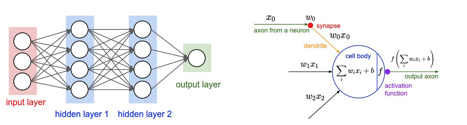
The following figures show the architecture of a neural network (left) and a single node (right).
The Fnn need a feature vector to train the network on. As we see from the figure, the size of the first
layer is the same size as our input feature vector.
We can convert small molecules to a feature vector by leveraging cheminformatics-based fingerprints
(Molecule OE Fingerprint). One should be
mindful of the relation between feature vector and the size of the input dataset. One such empirical relation was stated
by Hua et al. [Hua-2005]
For uncorrelated features, the optimal feature size is N−1 (where N is sample size).
As feature correlation increases, the optimal feature size becomes proportional to √N for highly correlated features.
We can also choose our cheminformatics features based on the nature of the physical property we are trying to predict. For
instance, as solubility is more of a local fragment property, keeping the minimum and maximum radii of the fingerprint on the lower
end yields better results. In contrast, properties where different fragments of the molecule interact more may benefit
from larger radius sizes.
Besides the cheminformatics features, we may also tweak machine learning hyperparameters.
Sets of Hidden Layers is of particular interest as it dictates
the number of nodes in each layer of the network. These hidden nodes allow the network to learn and exhibit nonlinear behavior.
Thus, if the total number of nodes is too low, it might be insufficient for the network to learn the prediction function.
However, large number of hidden nodes makes the network learn the training set very minutely, thereby losing its ability
to generalize.
In this case, it would perform poorly for unseen samples.
This conundrum of too small versus too large hidden layers is known as the underfitting and overfittting problem.
A simple rule of thumb to determine this is:
Nh = Ns/(a*(Ni+No))
Ni = number of input neurons. (Equals bit length p2)
No = number of output neurons. (1 for regression networks, >=2 for classification networks)
Ns = number of samples in training data set.
a = an arbitrary scaling factor usually 2-10.
In addition, parameters such as dropouts and regularizers
help with overfitting as well. Users can train on a set of dropouts, and can set a value for L2 regularizers in the
Neural Network Hyperparameter Training Option.
Dropouts act by randomly turning off a certain percentage of the node while training. This introduces nondeterministic properties
in the model, thereby generalizing it for unseen data.
Regularizers are a great way to prevent overfitting, that is, where the model learns too many details on the training set and is
unable to predict unseen molecules. While there are many techniques to regularize, R2 regularizers are smoother and converge easily.
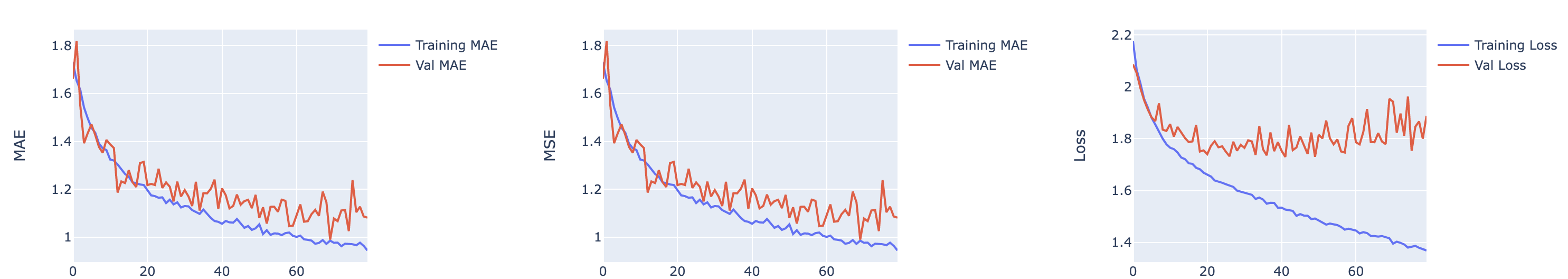
Here is an example of the training history of a model which suggests divergence.
Adding a regulizer would certainly improve the ability of the model to generalize.
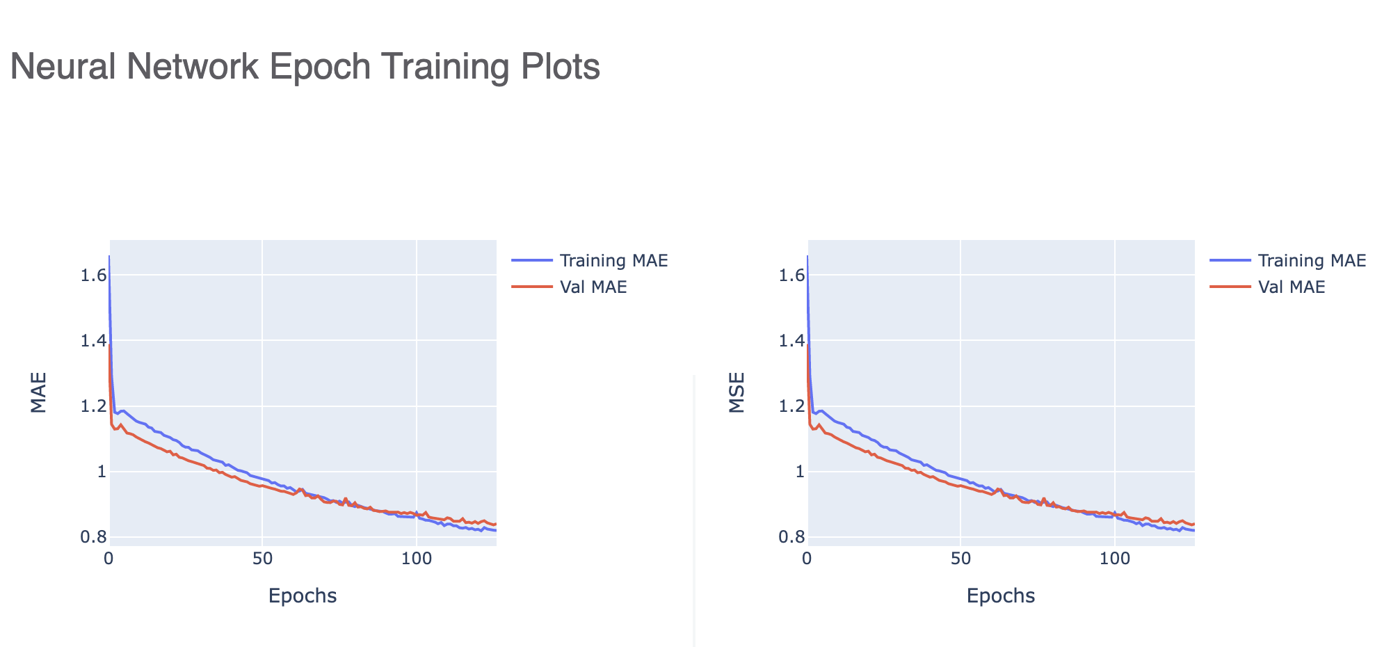
Once a model is trained, we can look into the training graphs in the Floe Report (Model Link) to gather more insight into
the quality of the model built. The graphs illustrate how the mean absolute error (MAE) and mean squared error (MSE) change
with every epoch of training. The first picture tells us that the learning rate is too high, leading to large fluctuations in every epoch.
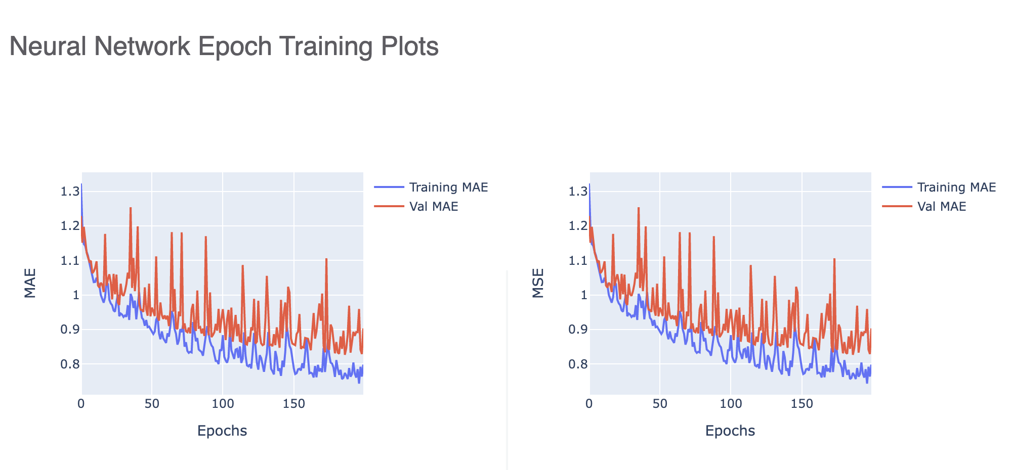
This one tells us that the validation error is much higher than the training, meaning we have overfit our model. Increasing
the regularization parameter or decreasing the number of nodes might be a good way to stop overfitting.
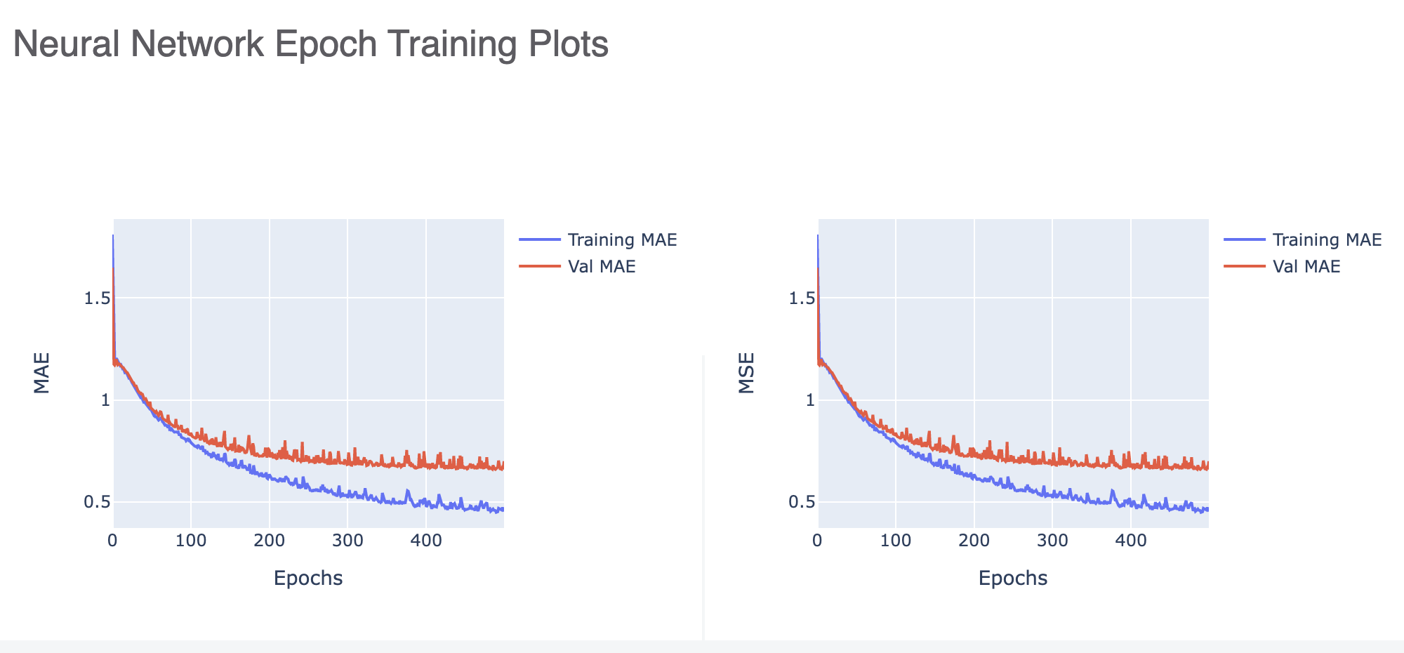
Finally, this picture shows us how a well-trained model should look.
A methodology called LIME (Local Interpretable Model agnostic Explanations)
explains machine learning predictions by learning a local interpretable model regarding the prediction.
It identifies the important bits in a fingerprint that are responsible for a certain prediction. These
bits are then mapped to individual parts of the molecules by finding the “core” atom using the bond degree of the query molecule.
The smallest pattern can be located and if there is a tie, a move to the larger “superset” patterns should be made.
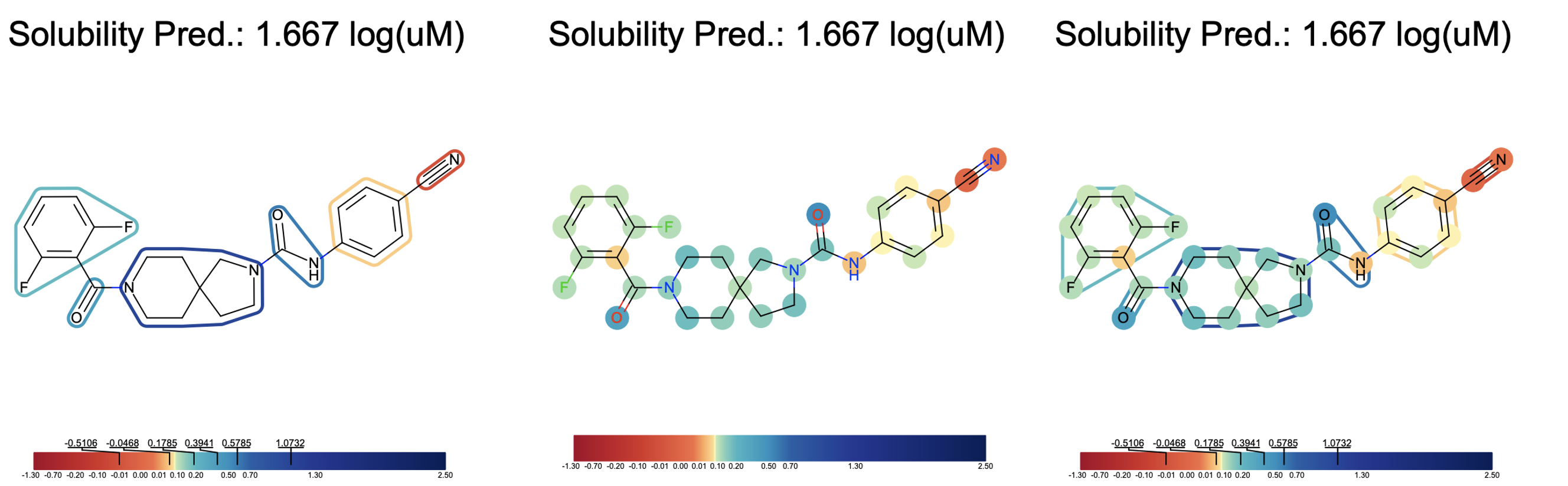
Shown below is an annotated image of a molecule with the bits that the algorithm thinks are important for the predicted property (solubility).
The bit importance can be translated to ligand or atom importance, and they can be annotated based on a color scale. Then
it is possible to view (a) annotated ligands, (b) annotated atoms, and (c) annotated ligand+atom explainer images as shown below.
Fragments such as amide bonds and hydroxyl groups are considered more soluble than the hydrophobic (greasy) benzene or nitrile
groups. Blue represents hydrophobic areas, red represents hydrophilic areas, and colors in between fall in the range between.
The models should be trained on different sets of fingerprints to see which explainer makes sense for the model.
The color schema can be adjusted using the QQAR. QQAR indicates
the quantile distributions of the LIME votes based on which the default color stops are defined. It allows the user to
put color stops on the color bar. By default, it is derived from the quantile of LIME vote distribution to give an even
color scale, but that can be changed to a more visually appealing scale if desired.