Edge Mapper for RBFE Calculations
A significant component of preclinical drug discovery involves optimizing the noncovalent binding between a target protein and ligands to improve affinity [Liu-2013]. To address this, many computational methods have been developed over the years; alchemical free energy methods are more expensive methods that target higher accuracy. These techniques can be used to compute either absolute binding affinities (ABFE) or relative binding affinities (RBFE). Although ABFE calculations are more attractive, RBFE calculations are more efficient and are therefore more widespread.
The RBFE approach requires a map of alchemical transformations between pairs of ligands; each transformation is known as an edge, and the entire set of transformations, or edges, must connect all the ligands together, forming a map that allows any ligand to be transformed into any other by following a path of edges (individual transformations). This map is generated prior to running the RBFE calculations. Starting from an Orion dataset of ligands, this tutorial uses the Edge Mapper for RBFE Calculations Floe in the MD Affinity Package to generate the map of edges needed for the RBFE calculations in the Nonequilibrium Switching Floe.
Given \(n\) ligands, out of all possible \(n(n-1)/2\) edges, the Mapper Floe selects a reasonable subset of the edges with the goal of keeping the computational demand low and providing a high probability of giving accurate RBFE calculations, considering each edge involves computational expense.
The OELOMAP is principally rooted in the Lead Optimization Mapper (LOMAP) [Liu-2013]. The general consensus is that the more similar the ligands in the edge are, the more accurate the free energy difference estimation is. Thus, edges are selected based on a set of heuristics for chemical similarity measures, including the MCS, ROCS®, and the equal charge check. All ligands should be part of a ring (cycle of edges) to provide a minimal redundancy of pathways to increase the accuracy of the RBFE calculations.
In the Map Type parameter on the Job Form, three map types are available in addition to the OELOMAP: a Star map with a center ligand (hub) ; a Binary Star map with two center ligands and an axle edge; and Multi-star map, which is a clustering-based perturbation map with multiple stars. If Star map or Binary Star map is selected, you are expected to provide the name(s) of the hub (reference) ligand(s), or the hub(s) will be automatically selected. If the specified hub ligand name(s) does not exist in the provided ligand set, it will also auto-select the hub(s). The choice of hub for a star map is the dominant factor in the performance of that map. It is currently under active development to find a good heuristic for the star map hub selection. Currently, for the star map, the representative parent molecule will be selected as a hub ligand and for the binary star map, the two hubs will be selected based on the similarities to other ligands.
The OpenEye Mapper Floe with its cubes and connections is shown in Figure 1.
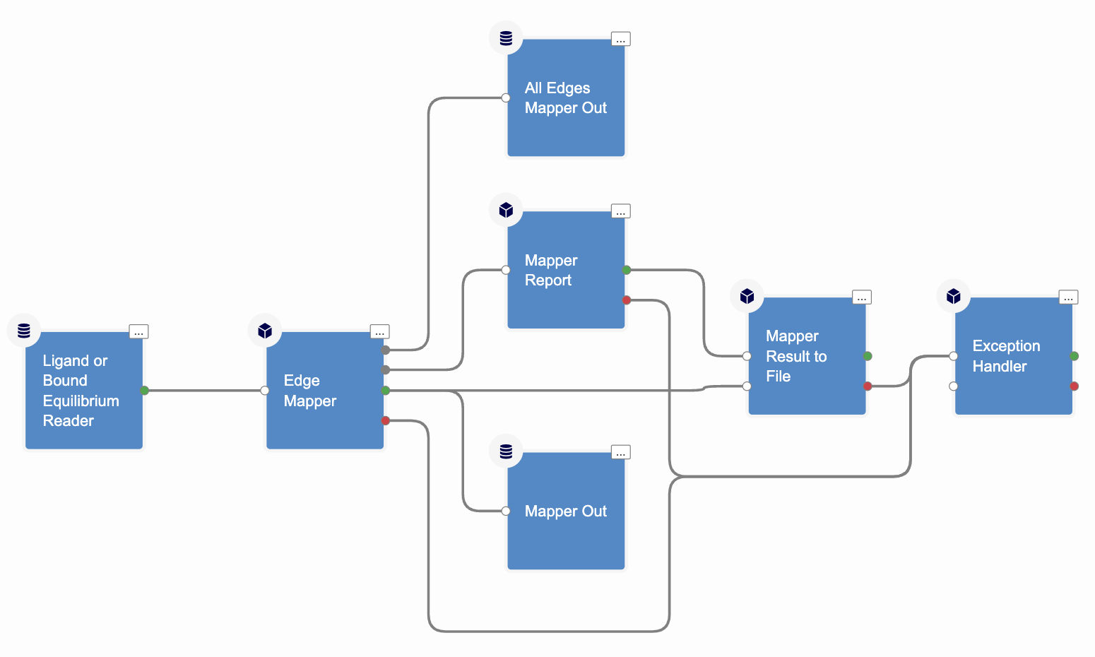
Figure 1. The Edge Mapper for RBFE Calculations Floe.
The Floe Inputs
To run the Mapper Floe, the usual input is an Orion dataset of posed ligands. The provided ligands must have reasonable 3D coordinates, all atoms specified, and correct chemistry such as bond orders and formal charges. This input ligand dataset could also be used as input for other protein-ligand MD floes such as the Bound Protein-Ligand MD, Short Trajectory MD with Analysis, or Ligand Bound and Unbound Equilibration for NES Floes; the output bound dataset produced by the Ligand Bound and Unbound Equilibration for NES Floe could also be used.
Optionally, you can also import an externally-generated map into the Mapper Floe to generate a Mapper output dataset of only those edges defined by the external map. In this case, the Mapper will not attempt to create the mapper graph, instead it simply translates the edges given in the user-defined file into the output dataset. However, the edge score is evaluated and displayed for the user-provided edges as well. The user-provided map must be a text file containing one edge per line in the following text format:
ligA >> ligB
The first field is the title of the starting ligand, followed by “>>”, and the third field is title of the final ligand. With the above example line, the Mapper will look in the input ligand dataset for a ligand titled “ligA” and another titled “ligB,” and it will generate an edge record in the Mapper output dataset defining the transformation of LigA into LigB. With user-defined maps, the ligand input dataset can contain ligands that are not used in any edge, but all user-defined edges must have ligands by that title in the input ligand dataset.
For this tutorial, the CDK2 receptor and sixteen ligands have been selected. The files can be downloaded below with the ligand mapping text file as well.
How to Use the Floe
Running the floe is straightforward. Figure 1 shows the Job Form for the Edge Mapper for RBFE Calculations Floe. Here, you can define the names of the job and the output datasets and select the Orion dataset of input ligands (for this tutorial, use the CDK receptor and ligand dataset you just downloaded). The Mapper will upload a .tar.gz file with useful information about selected edges as well as the edge information for all possible edges; you must specify this file name as well. In addition, you must set the name of the All Edges Mapper Dataset for all possible \(n(n-1)/2\) edges, which could be used in the Analyze page to select new sets of edges. If you want to run the floe using an external map file, you can specify it with the Optional Ligand Edge Map File parameter. For this tutorial, you may use the CDK2 ligand mapping file downloaded above. When using an external map file, the Mapper will not attempt to connect “similar” ligands to create edges, but it will only form edges based on those defined in the input map file.
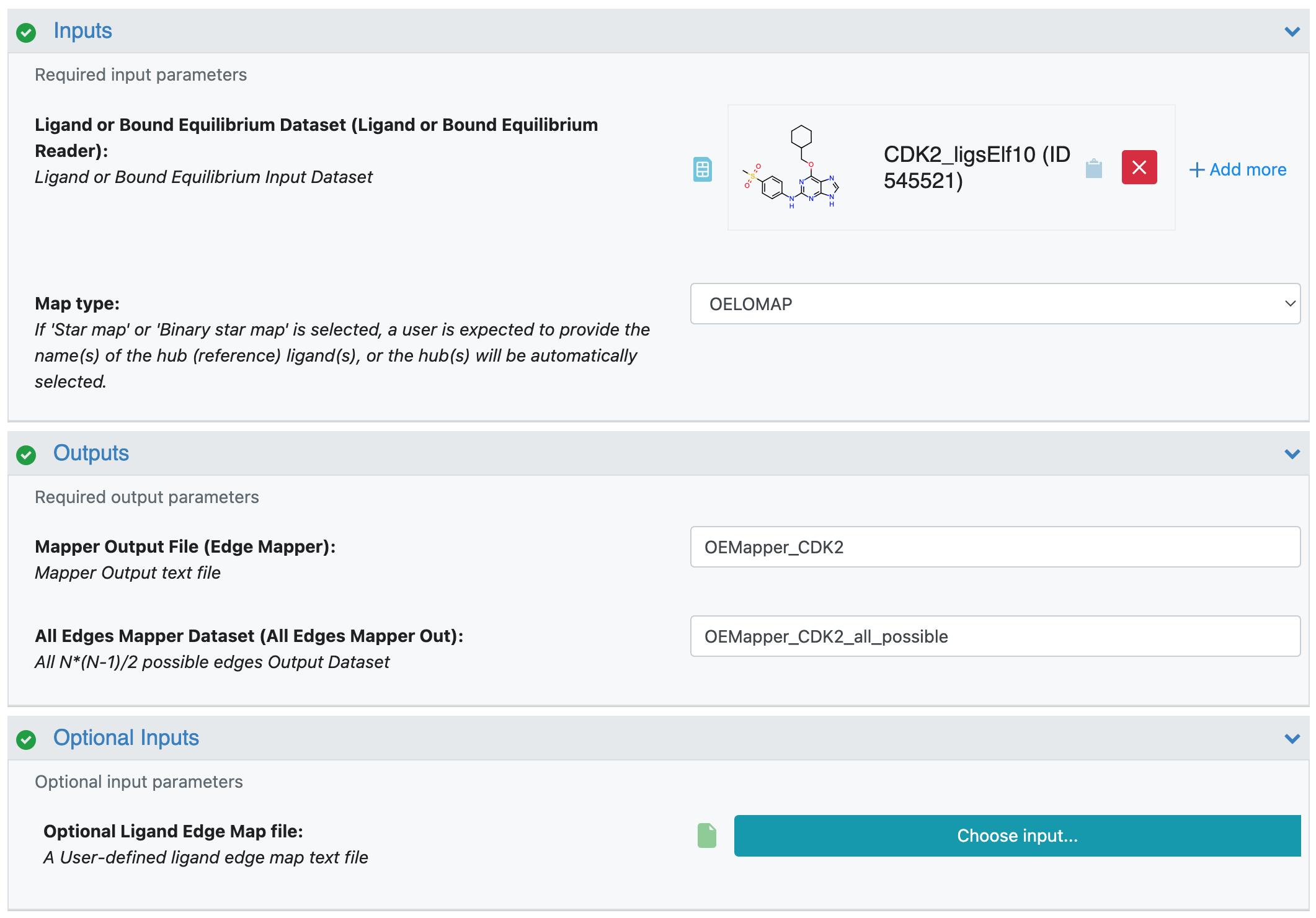
Figure 1. Job Form for the OE Mapper Floe.
At the end of the run, a Floe Report is produced with the generated map shown in Figure 2.
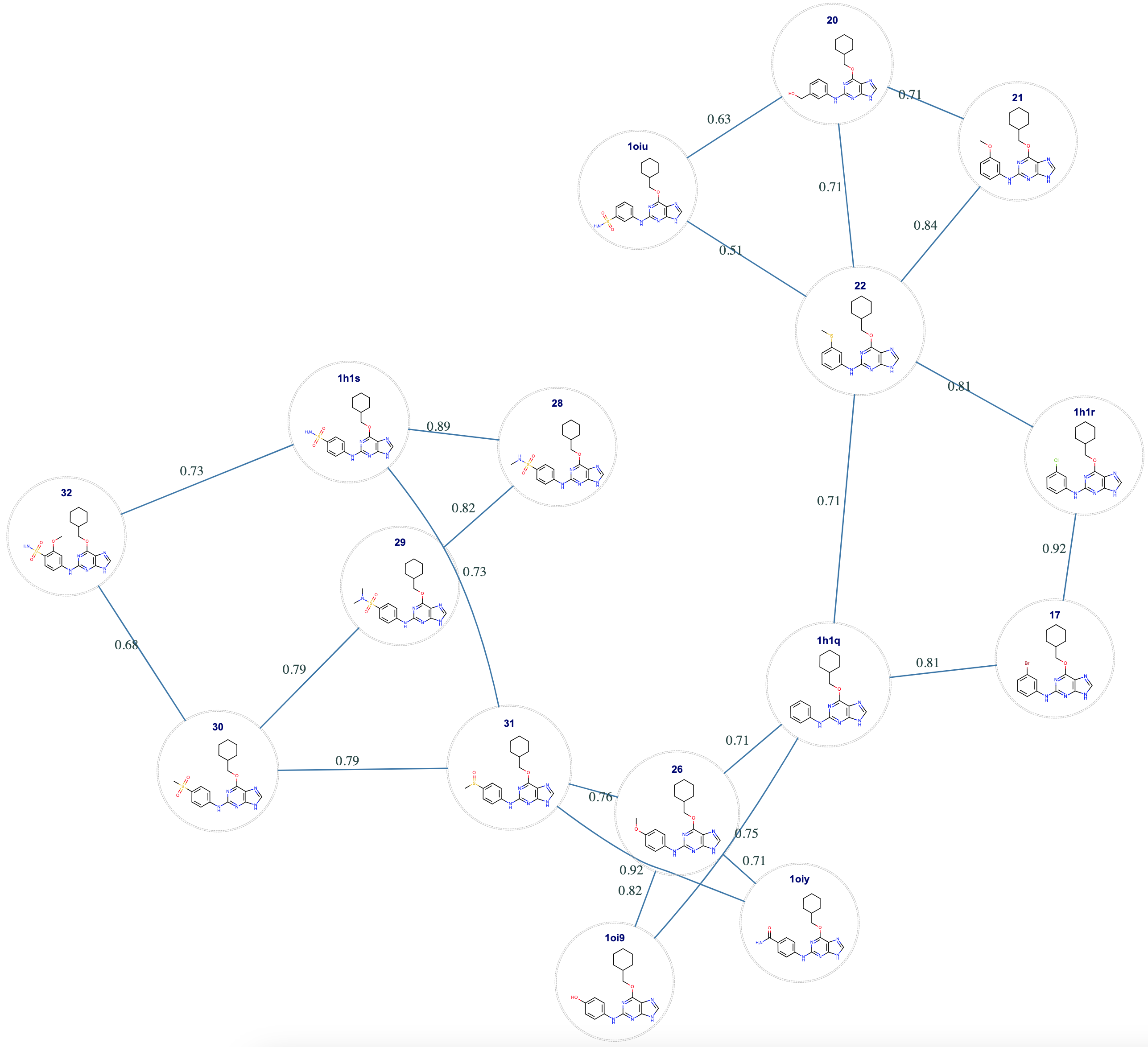
Figure 2. Map created by the Mapper tutorial.
Each edge in the graph is represented by a pair of ligands connected with a blue line. The float value with each line is the score computed by the Mapper for that edge. These scores are numbers in the range [0, 1] where zero is worst (i.e., this edge is unlikely to succeed) and 1 is best (likely to succeed). In addition to the graph diagram, two files are produced:
A map text file where each edge is tabulated according to the map file grammar previously described. This file can be downloaded and customized by adding or removing edges to make a user-defined input for a subsequent mapper run to make a custom map.
A .tar.gz file containing several edge information files: edges_by_ligand.csv, which contains lists of ligands connected to each ligand; LigA_LigB_edge_matrix.csv, which contains edges scores for all \(n(n-1)/2\) possible edges, Orion_record_fields_key.txt, which contains lists of fields of the output records; and lastly, the Floe report in a ZIP archive format. This could be useful in deciding which edges to add or remove in customizing the map. An example of the uploaded file can downloaded here:
How to Edit the Mapper Edges
Modifying and saving the customised edge map as a new dataset that can be used for the relative binding free energy calculations can be done in the interactive floe report.
On the bottom right of the floe report, one can find the help text which lists the available features for the modification. Please note that one should have access to the associated mapper output dataset to edit the edge map via interactive floe report.