Tutorial: pKa Exploration Floe
The pKa Exploration Floe enables you to explore the detailed predictions of micro- and macro-pKas along with related analyses such as titration curves, protonation microequilibria, speciation curves, and logD plots.
This floe also predicts all micro-pKa values for all possible microtransitions and subsequently calculates the corresponding macro-pKas. Using these micro- and macro-pKas, it generates individual detailed reports for each molecule.
The estimated cost of the pKa Exploration Floe run is approximately $0.01/molecule.
Running the Floe
Find the Floe
Click the “Floe” button on the navigation bar to reach the Floe page.
Click on the Floes tab.
From the Categories Floe Filters, click on the ‘Packages’ drop-down to expand the list of packages, then select the OpenEye pKa Prediction Floes package.
A list of the pKa Prediction floes will now be visible to the right. Select the pKa Exploration Floe.
Alternatively, you can enter the name of the floe in the search bar.

Figure 1. The brief description of the pKa Exploration Floe.
Click the “Launch Floe” button to open the Job Form.
Floe Parameters
Specify the parameter settings as indicated below.
Output Path: Select the path where you want to save output of this floe.
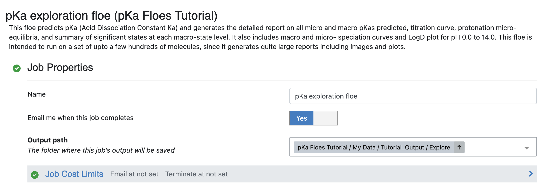
Figure 2. The output path for the floe.
Inputs
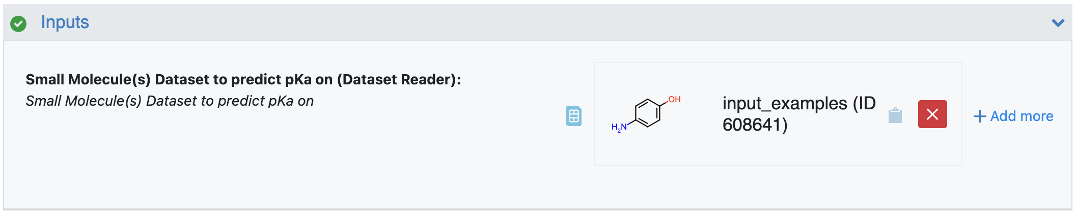
Figure 3. The tutorial input dataset.
Small Molecule(s) Dataset to Predict pKa On: This is the input dataset for the floe. Ionization states will be generated for the primary molecule on each record. For this tutorial, select ‘input_examples’ as the input dataset.
This example input dataset contains five molecules. Figure 4 shows the molecules in this dataset.
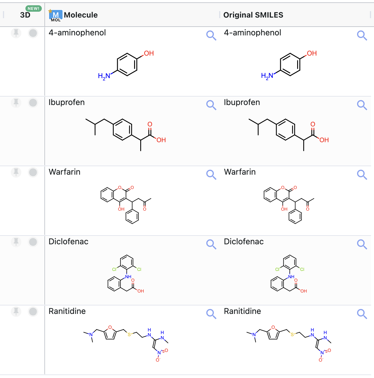
Figure 4. Structures of the molecules in the sample input dataset.
The sample pKa dataset for this tutorial can be downloaded here.
Input Example Dataset
Outputs
Specify the names of the output and failure datasets here.
Macro-pKa prediction: This output dataset contains macro-pKas and logD values at chosen environment pH values and links to the individual detailed pKa prediction report. Enter ‘tutorial_examples_macro_pKa’ for this tutorial. The other three output parameters are same as the output parameters described in the Generate Ionization States and Calculate LogD tutorial since this floe generates the same outputs of that floe. They are explained them here as well.
Significant Microstates: This parameter specifies the name of the output dataset which will contain significant microstates. For this tutorial, use ‘tutorial_examples_significant_states’.
Significant Ionization State Molecule Field: By default, the floe will replace the PrimaryMolField and use the name specified here to store the significant state of the molecule. If you do not want to modify the original PrimaryMolField, you can provide a new field name here and the floe will create an additional significant state field with this name. For this tutorial, a new field has been specified (see Figure 5).
Failed Descriptors Calculation: This parameter allows you to specify the output dataset of records where the floe failed to calculate descriptors. Here it is listed as ‘tutorial_examples_descriptors_failed’.
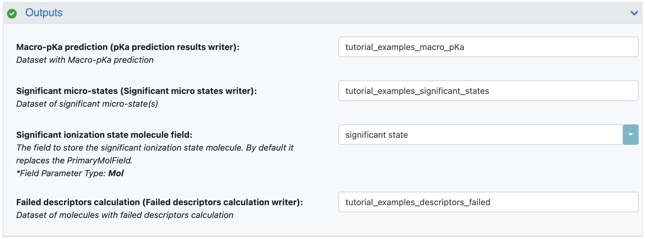
Figure 5. The floe output parameters.
Options
Get Multiple Significant States: By default, the floe will find only one most dominant ionization state. You can choose to save multiple significant states (if available). Turn this option On.
Calculate LogD: Use this parameter to select whether to calculate this value. By default, it is On.
Environment pH: By default, the floe has the environment pH set to 7.4, at which the floe will calculate the fraction of all ionization states and LogD. You can choose the environment pH to be anywhere from 0.0 to 14.0.
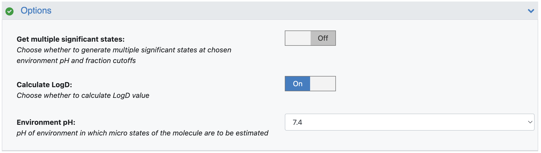
Figure 6. Filled parameters under the Options floe parameters.
Advanced Options
When all parameters have been set, click the “Start Job” button to run the floe.
Floe Run Overview
The job should finish in a few minutes. It predicts pKa values and creates a floe report with information about each molecule including predicted macro-pKas. The output dataset includes a link for each record to the associated part of the report. Figure 7 shows that the floe generated one significant state, for each of the five input molecules, since we opted NOT to save multiple significant states in this floe run. In addition, the molecule descriptor calculation did not fail for any molecules.
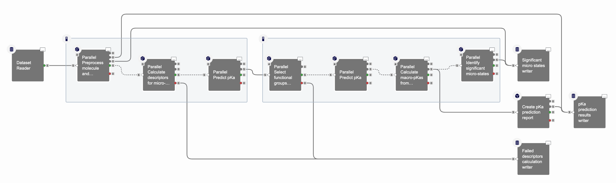
Figure 7. An overview of the cubes in the completed floe.
Floe Output Dataset
There should be two output datasets for successful predictions.
‘tutorial_examples_macro_pKa’: This dataset contains macro-pKas, logD at chosen environment pH and link to the individual detailed pKa prediction report. It has a single record entry for each molecule.
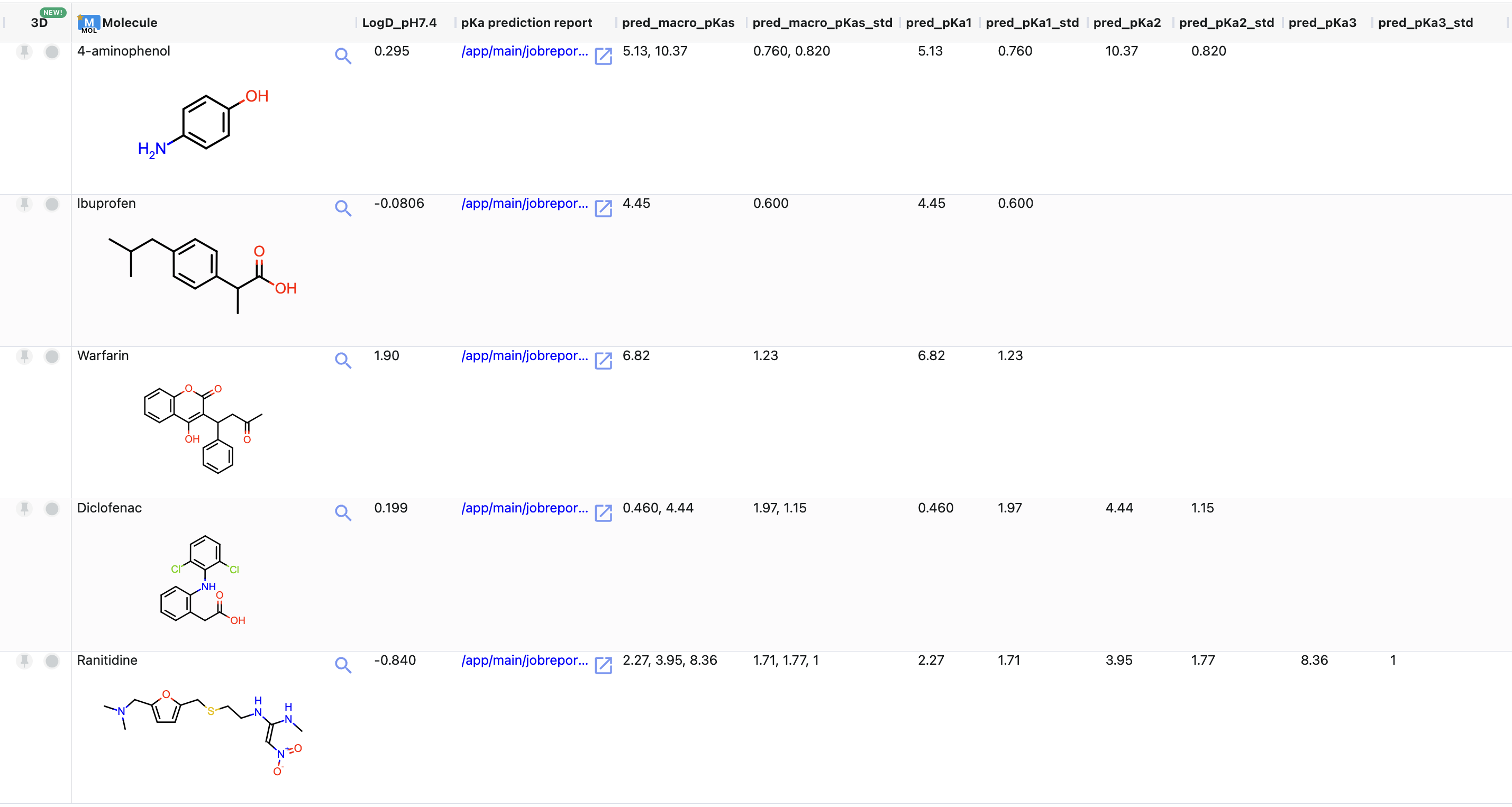
Figure 8. The floe output dataset.
‘tutorial_examples_significant_states’: This includes the same output generated by the Generate Ionization States and Calculate LogD Floe. It is explained in the tutorial for that floe.
pKa Prediction Report
The main purpose of this floe is to dive deeper into the micro- and macro-pKa prediction. For that, this floe generates a detailed floe report with a page for each molecule. The following sections explain each part of those pages.
Index Page of All Molecules
The page for a given molecule can be accessed from its record in the tutorial_examples_macro_pKa dataset, an index page is provided with all molecules run in this job. It has a grid view of the structures of all molecules that are linked to individual pages. To limit the size, the index page shows a maximum of 1000 molecules. The remaining molecules can still be accessed through links provided in the Macro-pKa Prediction dataset (‘tutorial_examples_macro_pKa’, in this case).
Click on one of the image tiles to open the report (or open it from the dataset). Figure 9 shows an example report of 4-aminophenol.
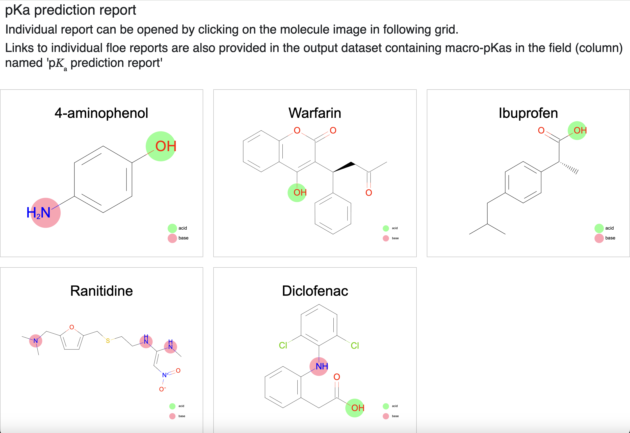
Figure 9. The pKa prediction floe report.
Molecule Page Table of Contents and Dominant Ionization State
The first section is divided into two columns. The left side is a table of contents with hyperlinks to jump to all sections of the page, and the right side shows the dominant state of the given molecule at the chosen environment pH. In this case, it shows the dominant state of 4-aminophenol at pH 7.4. It also highlights the identified ionizable groups as acidic (light green) or basic (light pink).
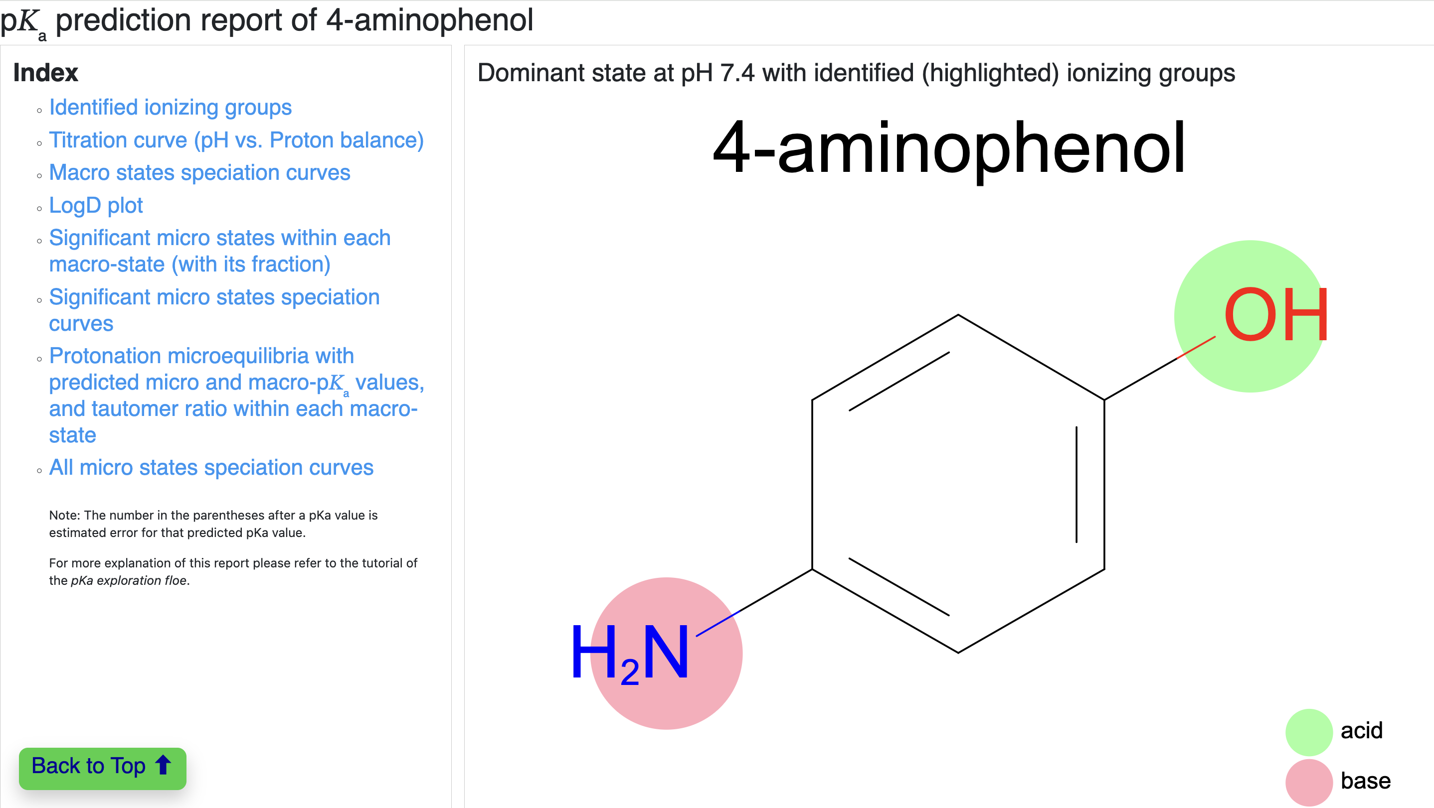
Figure 10. The individual pKa prediction report index for the dominant ionization state of 4-aminophenol.
Titration Curve
The next section shows the titration curve generated from predicted macro-pKas. It shows the proton balance on the X-axis versus the pH (from 0 to 14) on the Y-axis. Hovering a mouse over the titration curve shows the corresponding pH and proton balance. It also marks the predicted macro-pKas within the range of 0 to 14.
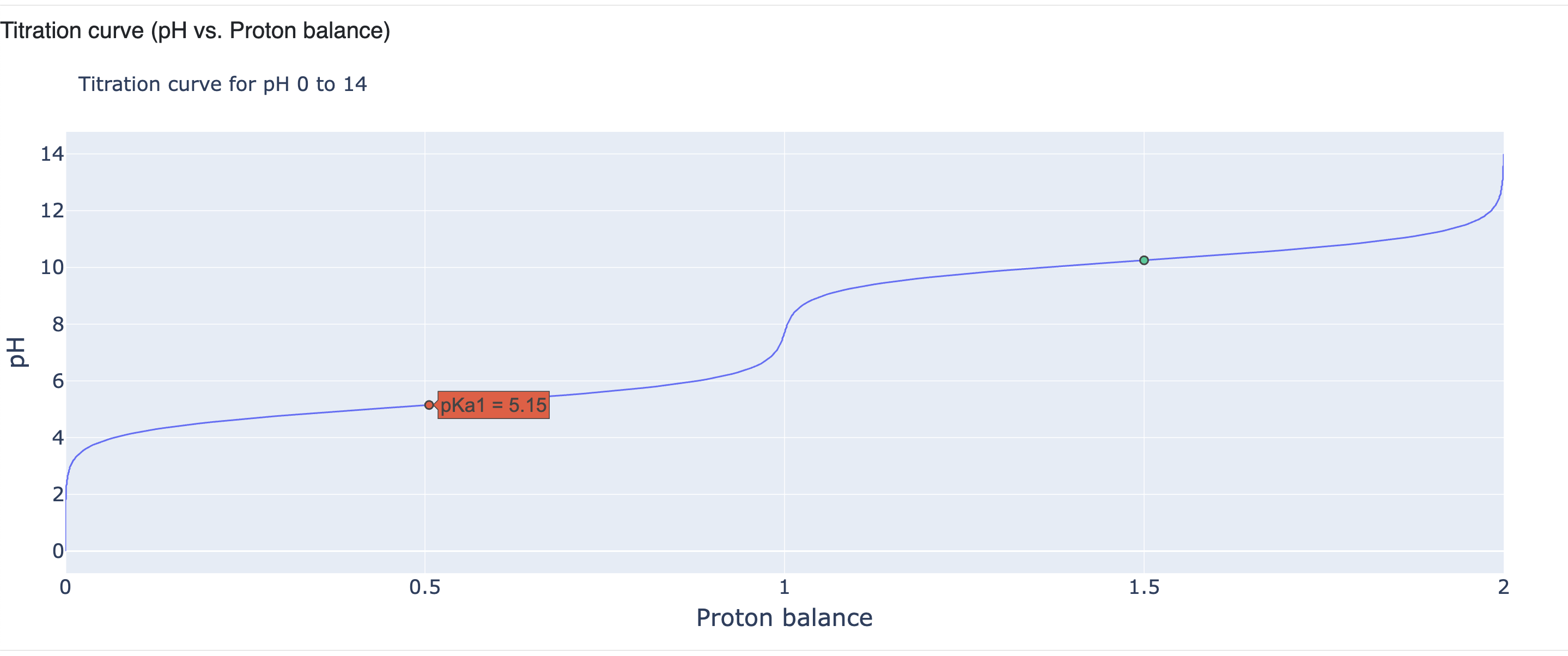
Figure 11. The titration curve for the dominant ionization state of 4-aminophenol.
Macrostate Speciation Curves
The next section includes speciation curves of the macrostates for pH values from 0 to 14. The plot is interactive and shows the fraction of all macrostates (in percent) by hovering on any pH in the plot. In this example, the current hovering view shows the fraction of all macrostates at pH 7.4. The plot shows that the macrostate H2M+ is most dominant from pH 0 to nearly 4 and then begins to decline as the presence of the macrostate HM increases. At approximately pH 5.15, they both reach nearly 50% prevalence. The macrostate M- is still present in a negligible amount. At pH 7.4, the macrostate HM is dominant (~99%) and the other two macrostates, H2M+ and M- are present as less than 1%. The macrostate M- starts to increase after pH 8 and becomes dominant as the pH rises to 11 and then to 14.
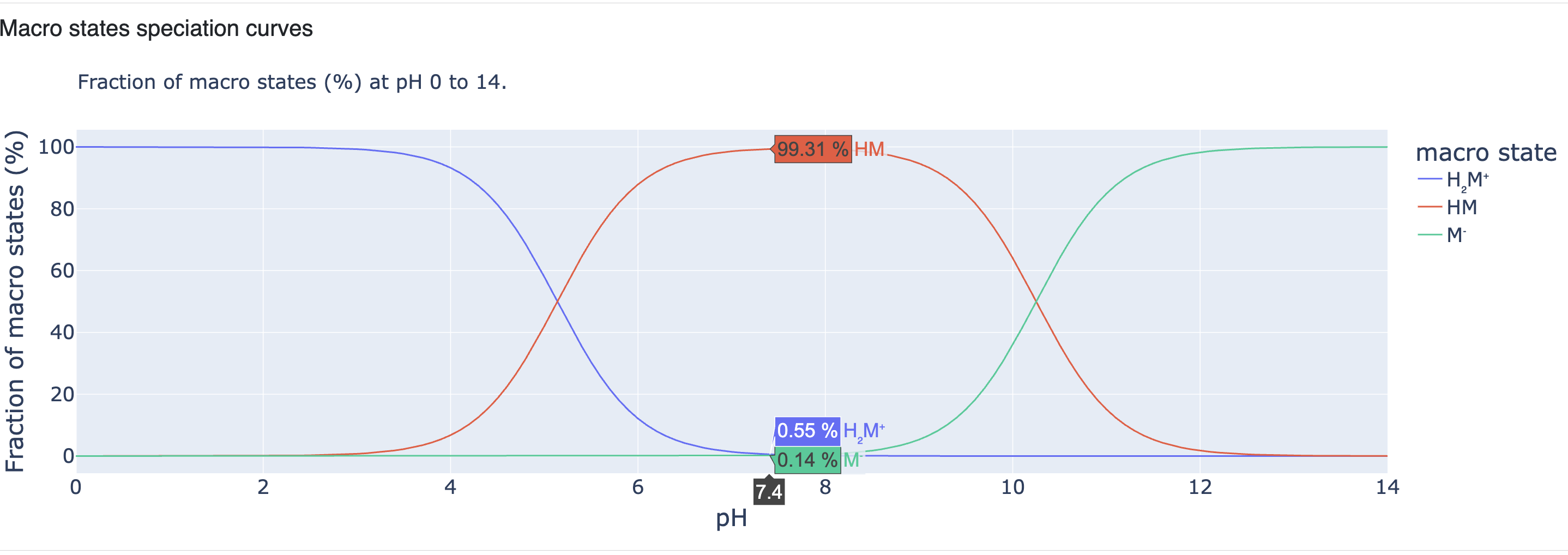
Figure 12. Macrostate speciation curves.
logD Plot
Now that we have predicted the pKa and the calculated fraction of each micro- and macrostate from in pH 0 to 14, we can calculate LogD at any pH at from 0 to 14. LogD is calculated from the XLogP of un-ionized molecules and the calculated ratio of un-ionized and ionized fractions of the molecule at any given pH. Based on that, the following LogD plot for pH 0 to 14 is calculated.
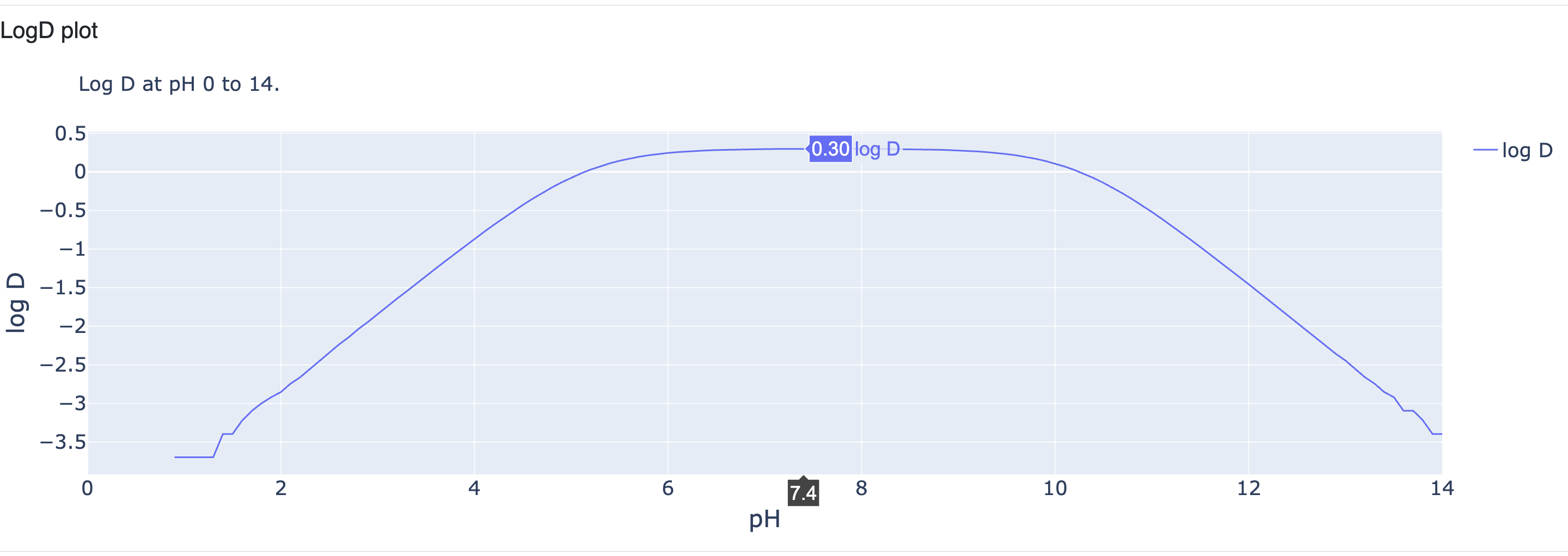
Figure 13. The LogD plot.
Significant States per Macrostate
We have already seen the macrostate speciation curves (% macrostates for a given pH from 0 to 14). But it can also be useful to know which microstate was the most dominant in each macrostate when considering all functional groups to be fully protonated in order to reach a fully deprotonated state. Figure 14 shows the significant states for each macrostate and the corresponding macro-pKa for each macrostate transition from fully protonated to fully deprotonated. This image also shows the deprotonation of ionizing groups that were not selected to be processed in the detailed micro- and macro-pKa predictions. The image in the top right corner is the un-ionized form of the molecule as a reference.

Figure 14. The significant states within a macrostate.
This is a simple example shown here for the purpose of this tutorial. But if a molecule has multiple significant states possible within one macrostate (net charge), then those are all shown in this image at the corresponding macrostate level. Figure 15 shows an example of ranitidine (from this tutorial’s example input dataset). This image shows only macrostates where multiple significant microstates were possible and were reported in Figure 14.
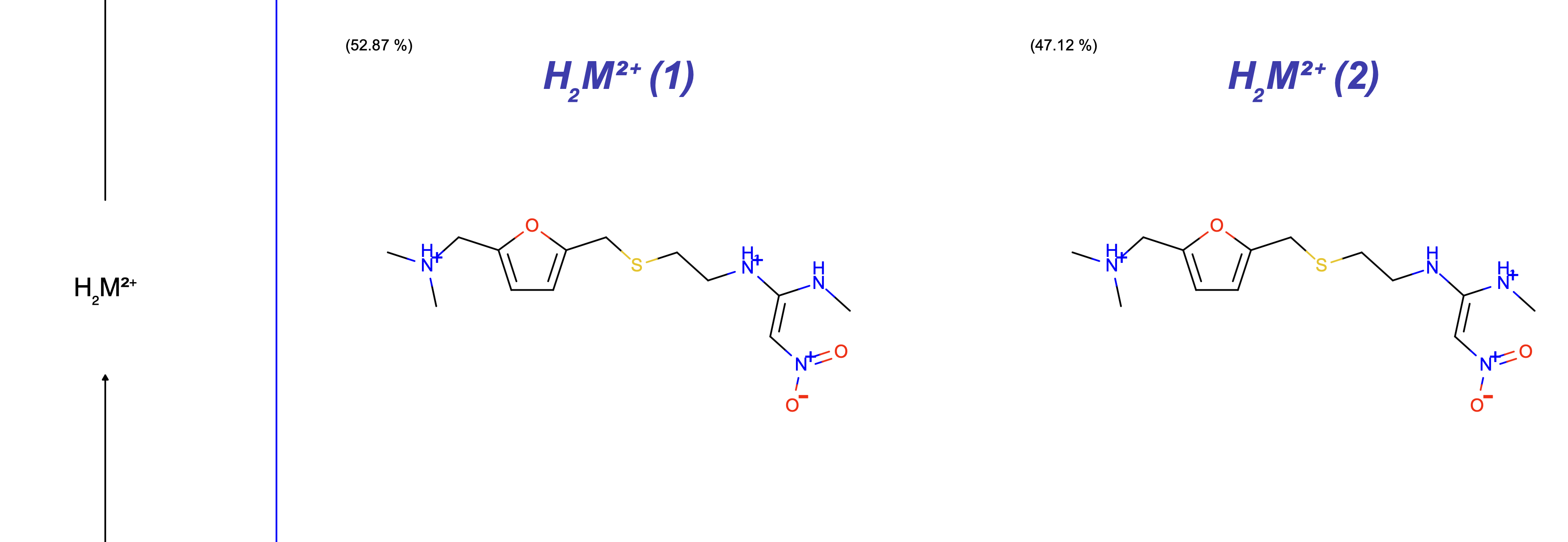
Figure 15. A ranitidine example with multiple significant states per macro state.
Figure 16 shows the expanded version of the ranitidine example in Figure 15.

Figure 16. Significant states per macrostate for ranitidine.
Significant Microstates Speciation Curves
The fraction percentage of significant microstates shown in Figure 14 are also displayed here as speciation curves from pH 0 to 14 (Figure 17).
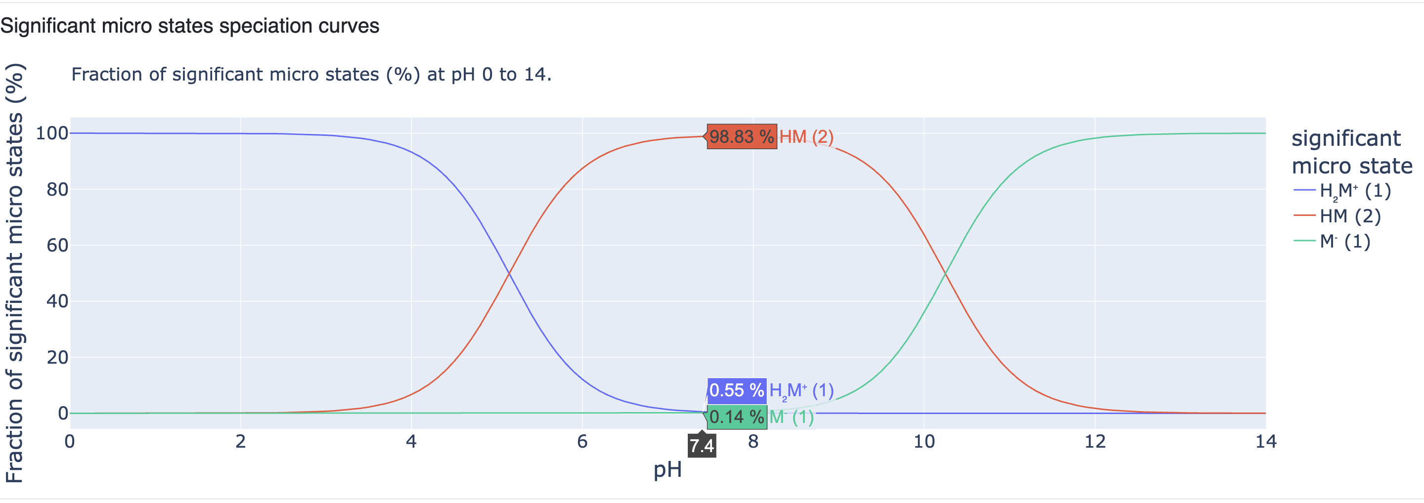
Figure 17. Significant microstates speciation curves.
Protonation Microequilibria
The detailed protonation microequilibria are displayed in this section. The top row shows macrostate transitions from the fully protonated form (highest net charge) to the fully deprotonated form (lowest net charge). The macrostate labels are shown at the end of the macrostate transitions, and macro-pKas are shown on the arrow specifying the macrostate transition. Below that, detailed protonation microequilibria are displayed along with micro-pKas displayed on each arrow (microtransition). The value in parentheses shows the prediction error. The ionizing groups are highlighted in light green if they are protonated and in light pink if they are deprotonated. The bar on the left of each microstate shows its fractional percentage within that macrostate. For example, the microstate H2M+ (1) is the only single microstate within the macrostate H2M+. So, that contributes 100%. But in the case of the macrostate HM, there are two possible microstates: HM(1) (zwitterion) and HM(2) (neutral). Here, the calculated fractions displayed as bar shows that the zwitterion form is present in a negligible amount while the neutral form contributes >99%.

Figure 18. Protonation microequilibria.
Occasionally, a molecule with too many ionizable groups or with groups that have an extreme intrinsic pKa value is given as input to the pKa floes. In this case, the FAQs discuss how those ionizable groups can be treated. In addition, this example shows protonation microequilibria that are generated with an unselected ionizing group for detailed micro- and macro-pKa prediction.
All Microstates Speciation Curves
This plot displays speciation curves for all microstates (not just significant ones).
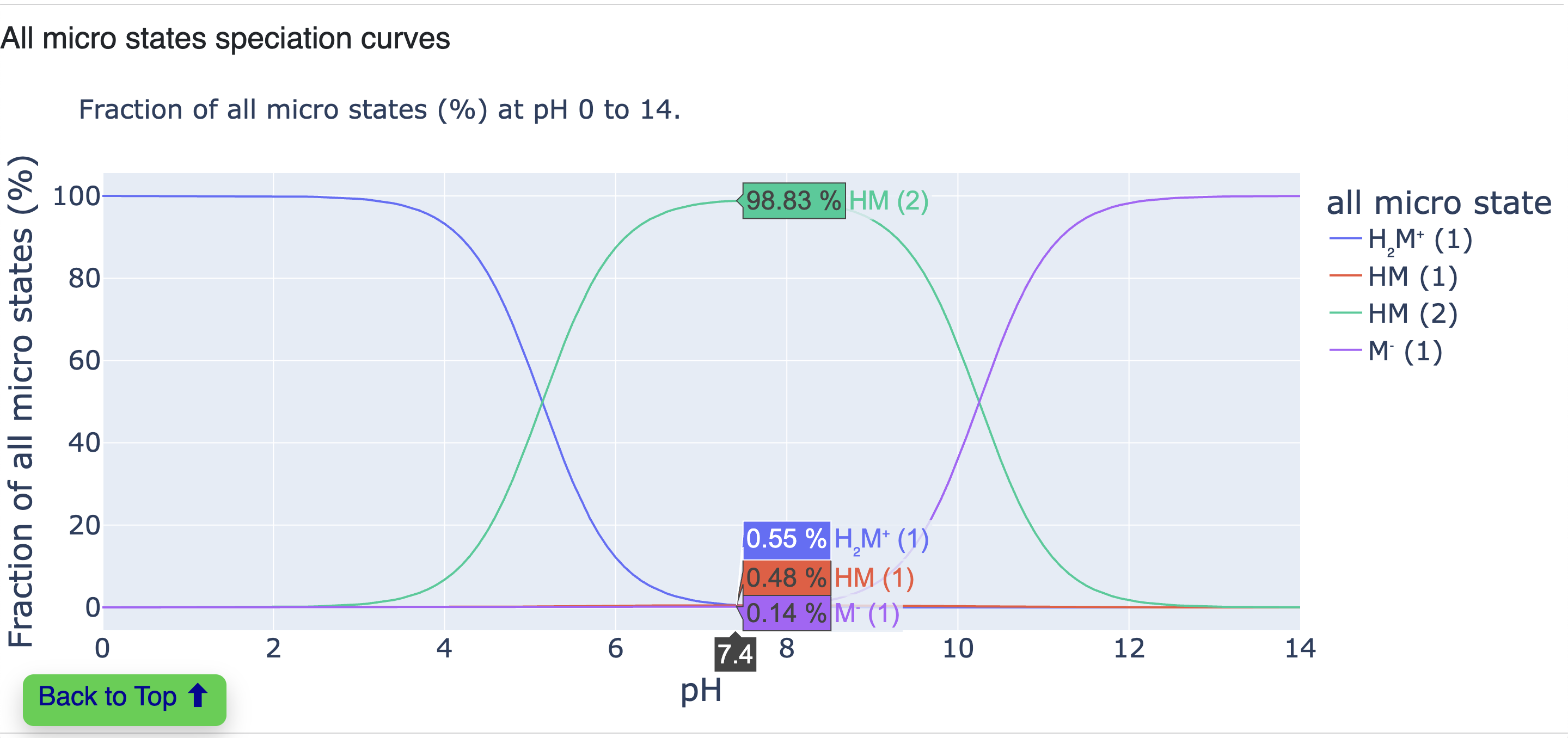
Figure 19. Speciation curves for all microstates.