Soup to Nuts Tutorial: A Real Application Example of HER2
This tutorial shows how to use the Structural Biology Floes to perform a “soup to nuts” analysis on real cryo-EM data starting with a protein structure and cryo-EM data and moving to a pocket ready for high-throughput virtual screening extracted from our cryo-EM-driven simulation.
You will:
Prepare a protein structure PDB file for simulation.
Simulate the protein using weighted ensemble MD (WEMD) with a progress coordinate defined using a heterogeneous map from the conformational heterogeneity analysis of a publicly available particle stack.
Use the Cryptic Pocket Detection Floes to find pockets opened during our cryo-EM WEMD exploration.
But first, let’s discuss the test system.
HER2-Trastuzumab-Pertuzumab Complex
The PDB deposition 8PWH is the structure of the human epidermal growth factor receptor 2 (HER2) and the antigen-binding fragments from two distinct therapeutic antibodies, trastuzumab and pertuzumab (referred to as HTP in the complex). HER2 plays an important role in cell signaling, and its deregulation is implicated in the pathologies of various cancers. Pertuzmab and trastuzumab are both humanized monoclonal antibodies, approved by the FDA for the treatment of HER2-positive breast cancer.
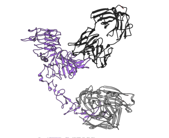
Figure 1. The PDB 8PWH structure, with HER2 shown in purple, trastuzumab and heavy chains in light grey, and pertuzumab and heavy chains in dark grey.
This protein structure was published as part of a study by Bressanelli, et al., in which they performed two types of heterogeneity analysis (3DVA and MDSPACE) on cryo-EM data to study the conformational heterogeneity of the HTP complex [Bressanelli-2024]. PDB 8PWH is the protein structure refined in the composite reconstruction from the authors’ analysis of the cryo-EM particle stack.
The authors of this study also deposited their particle stack in the Electron Microscopy Public Image Archive (EMPIAR), under the deposition access code EMPIAR-11665. Using this particle stack, we ran a separate algorithm for analyzing the heterogeneity present in the particle stack, called RECOVAR.
Note
We prefer RECOVAR to 3DVA due to its advanced regularization techniques and the fact that
it outperformed almost all other techniques (including SOTA machine learning techniques)
in the recent CryoBench benchmarking paper.
This gave us an opportunity to check our own analysis for consistency, by
comparing the heterogeneity we observe with the published account of
heterogeneity reported in the Bressanelli study. RECOVAR can be pip-installed following
the directions in the github repository above.
If you prefer to skip the RECOVAR analysis portion below, please download
all_init_files.tgz, expand it locally, and
upload the files under the her2 folder to Orion.
RECOVAR Particle Stack Analysis
The particles can be downsampled from 280x280 to 256x256 pixels (the maximum recommended image size for RECOVAR analysis) using cryodrgn:
cryodrgn downsample -D 256 -o HER2_downsampled_256.star --outdir ./HER2_downsampled_mrcs_256/ --datadir ${PATH_TO_EMPIAR_DIR}/11665/data/extract/ ${PATH_TO_EMPIAR_DIR}/11665/data/J503_csparc2star-particles.star
cryodrgn parse_pose_star ${PATH_TO_EMPIAR_DIR}/11665/data/J503_csparc2star-particles.star -o poses.pkl -D 256
cryodrgn parse_ctf_star ${PATH_TO_EMPIAR_DIR}/11665/data/J503_csparc2star-particles.star -D 280 --Apix 1.16 -o ctfs.pkl
Then, from the HER2_downsampled_mrcs_256/ directory, you can run:
recovar pipeline --outdir recovar_output_low_memory --poses ../poses.pkl --ctf ../ctfs.pkl --lazy --low-memory-option --datadir ./ HER2_downsampled_256.star
–lazy and –low-memory-option are necessary on systems for which the RAM is insufficient to store the whole particle stack at once.
Once the pipeline analysis is complete, you can view the mean map and eigenmaps from the PCA analysis in the recovar_output_low_memory/outputs/volumes/ directory. The eigenmaps are three-dimensional analogs of eigenvectors in standard linear algebra; that is, in the PCA decomposition of the heterogeneity present in the particle stack, the eigenmaps represent the the direction of largest variance, sorted by the magnitude of their eigenvalues, with eigen_pos0000.mrc being the largest and eigen_pos0001.mrc being the second largest. Below,you will use the Automated WEMD Simulation and Best Structure Search Guided By Eigen CryoEM Maps Floe to project the dynamics observed in simulation onto these eigenmaps, to see where the heterogeneity is consistent with them.
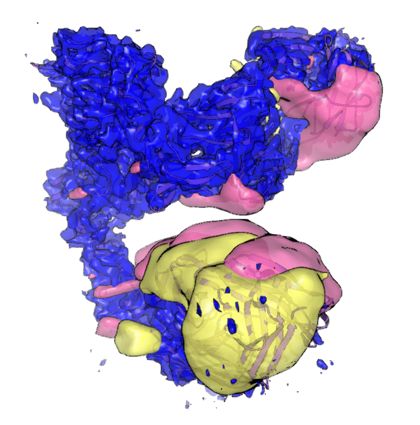
Figure 2. The mean map from RECOVAR analysis (blue) at a contour level of 0.01, with eigenmaps 0 (pink) and 1 (yellow) at contour levels of 5E-7.
Below is the UMAP projection from RECOVAR analysis of the EMPIAR 11665 particle stack. This figure is a representation of the heterogeneity estimated from the 750,000 particles in the deposited particle stack, across the ten latent dimensions used in analysis and projected onto two dimensions.
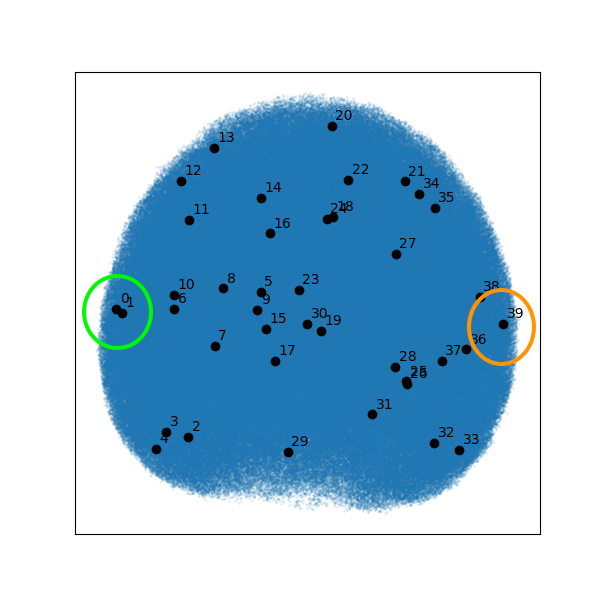
Figure 3. UMAP projection of the heterogeneity in the particle stack from EMPIAR-11665 analyzed by RECOVAR. See the k-means cluster center 0 on the left and 39 on the right.
The UMAP projection finds a low-dimensional representation of the nearest-neighbors graph in higher dimensions (in this case, the ten dimensions from the PCA analysis) whose edge probabilities in the low-dimensional graph are as similar to the high-dimensional graph as possible. Thus, scatter points closer together in the UMAP projections should be closer together in the higher-dimensional latent space (and vice versa for points farther apart).
You can compute the densities from each of the k-means cluster centers, using:
recovar analyze ./recovar_output_low_memory/ --zdim=10
Or, to save time, simply compute the density associated with the cluster centers of choice by isolating the latent space coordinates of that cluster center from the /analysis_10/kmeans_center_coords.txt file on their own, for example, using center_0.txt file and running:
recovar compute_state ./recovar_output_low_memory -o center_0/ --latent-points center_0.txt
The volumes have been extracted from k-means clusters 0 and 39 in Figure 3 above, and they are shown below, superimposed onto the mean map from RECOVAR analysis. Notice the heterogeneity seemingly present in the trastuzumab and pertuzumab regions of the map (a kind of “breathing” motion bringing the antigen binding domains closer together and further apart). This is the heterogeneity you will attempt to model in simulation.

Figure 4. K-means cluster center map 0 (green) and 39 (orange) from RECOVAR, alongside the mean map from RECOVAR (blue). Notice the differences in the trastuzumab region on the bottom and the pertuzmab region on the top right. Compare this with the heterogeneous maps representing heterogeneity in the trastuzumab region from the 3DVA and MDSPACE analysis from the Bressanelli study [Bressanelli-2024].
The resolution of the maps produced by RECOVAR is between 3.5 Å and 4 Å, so specify a consistent resolution of 3.7 Å in all of the floes below.
In this tutorial, you will use the Structural Biology Floes to start from the PDB deposition 8PWH; extract simulated structures consistent with k-means cluster centers 0 and 39 from RECOVAR using the Automated WEMD Simulation and Best Structure Search Guided by Target CryoEM Map Floe; and explore the space of heterogeneity from the two largest eigenvalue PCA dimensions using the Automated WEMD Simulation and Best Structure Search Guided By Eigen CryoEM Maps Floe.
SPRUCE Protein Preparation
Start by preparing the system with SPRUCE.
The SPRUCE - Protein Preparation Floe requires only the PDB ID as input. However, given that the output dataset will be used as the input to the molecular dynamics simulation, you should change two additional parameters.
Outputs
Output All Biological Units: Toggle this on. This will output the intermediary structures in SPRUCE’s design unit preparation that serve as valid input structures to the Solvate and Equilibrate Target Protein Floe.
Unliganded Structure Parameters
Enumerate Pockets: Toggle this off because it is unnecessary to search pockets based solely on the deposited structure from the PDB ID.
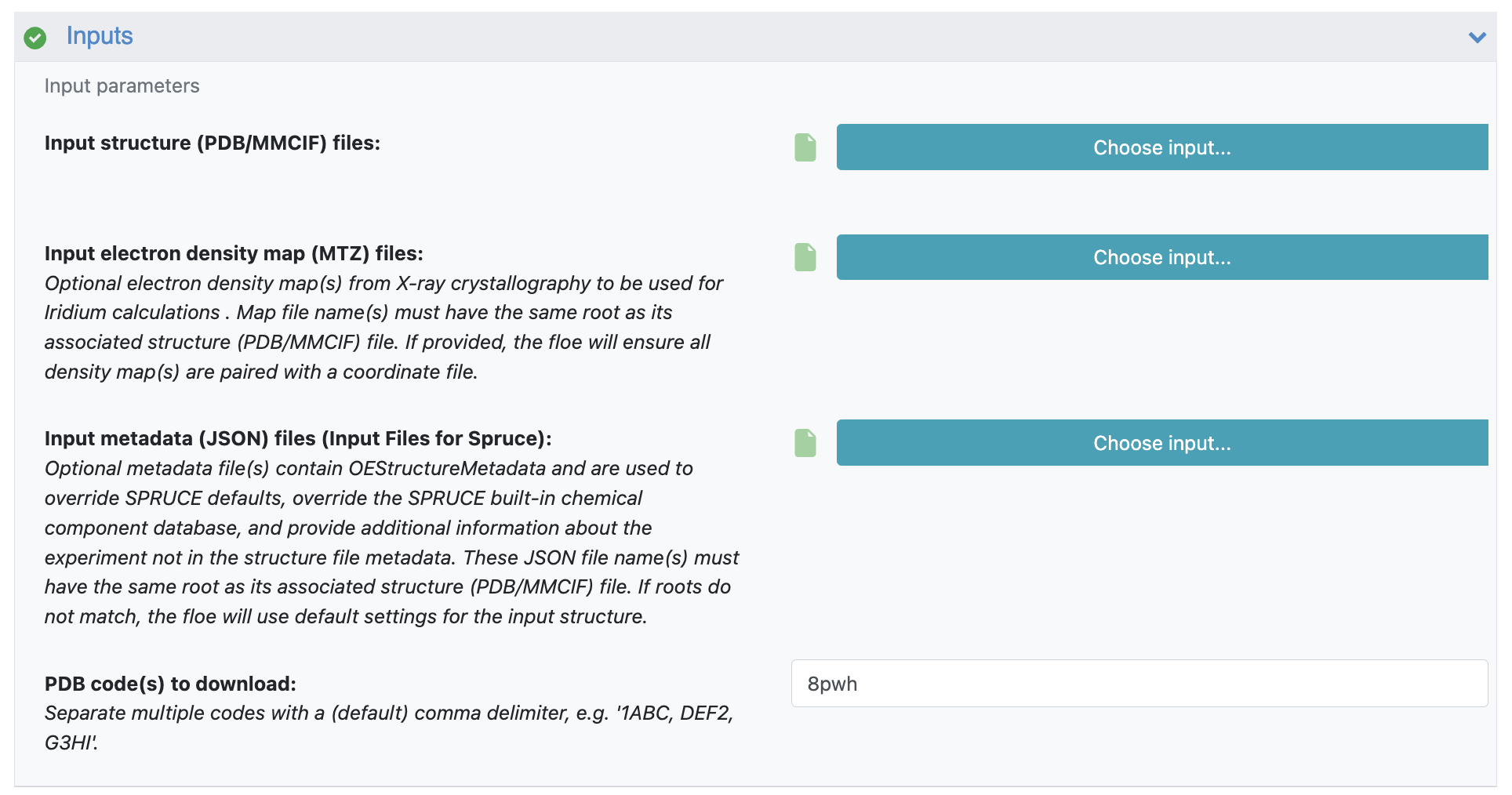
Figure 5. Inputs for the SPRUCE - Protein Preparation Floe used to prepare the PDB deposition 8PWH.
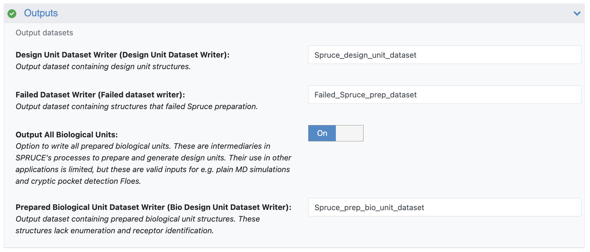
Figure 6. Toggle Output All Biological Units on because the output structure will be input to an MD preparation floe.
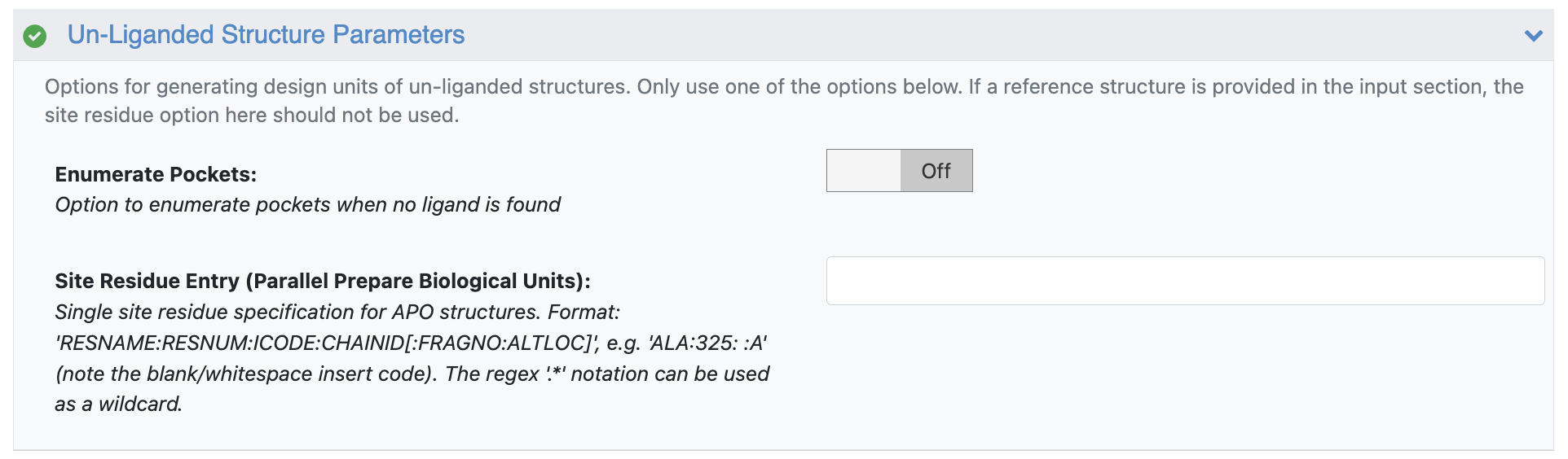
Figure 7. Toggle Enumerate Pockets off to avoid searching pockets based on the single structure of 8PWH.
Note
The SPRUCE - Protein Preparation Floe should take less than 10 minutes to run and cost well under one dollar. It will take longer when the Enumerate Pockets parameter is toggled on, but the floe will try to find all possible pockets based on the single structure of 8PWH and will output a design unit dataset with each design unit consisting of one receptor and one pocket. This dataset is used as input to the Solvate and Equilibrate Target Protein Floe as described below.
Simulation System Preparation
Next, the Solvate and Equilibrate Target Protein Floe will be used to prepare the protein for simulation. This floe requires only the output biological unit dataset from SPRUCE as input.
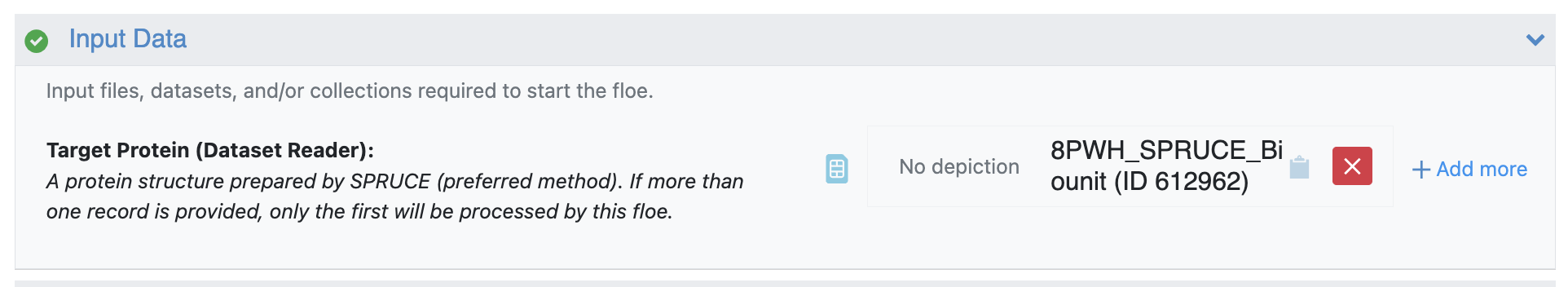
Figure 8. The output dataset from the SPRUCE - Protein Preparation Floe is used as input for the Solvate and Equilibrate Target Protein Floe.
Note
The Solvate and Equilibrate Target Protein Floe should take approximately 4 hours to run and cost less than $15.
Simulation Using the Automated Best Structure Search Floe
The Automated WEMD Simulation and Best Structure Search Guided by Target CryoEM Map Floe takes the output dataset from the Solvate and Equilibrate Target Protein Floe as input. This floe runs a weighted ensemble molecular dynamics (WEMD) simulation with a progress coordinate based on the real-space correlation coefficient (RSCC) between the consensus or target map of your choice and maps simulated on the conformation sampled in every frame of simulation. Though the progress coordinate is defined with respect to the target map, the protein might sample conformations consistent with other maps as well: the progress coordinate is necessary to define the progress coordinate space the simulation explores. This automated floe will output the conformations sampled in a simulation that are most consistent with the number of maps the user inputs, allowing for production of structures consistent with many maps from heterogeneity analysis simultaneously.
For simplicity in this tutorial, perform the simulation with respect to k-means cluster center map 0 and output the best structure search conformations for both k-means cluster center maps 0 and 39. Please note, however, that any number of maps can be input (for example, all outputted by RECOVAR with default settings) to the Input Cryo-EM Maps and Options for Best Structure Search parameter group, with minimal added cost.
Start with a short five-iteration test, to ensure that the results look reasonable, before moving to a longer (e.g., 50–100 iterations) simulation using the Continue WEMD Simulation Guided by CryoEM Maps Floe.

Figure 9. The output dataset from the Solvate and Equilibrate Target Protein Floe is used as the input dataset.
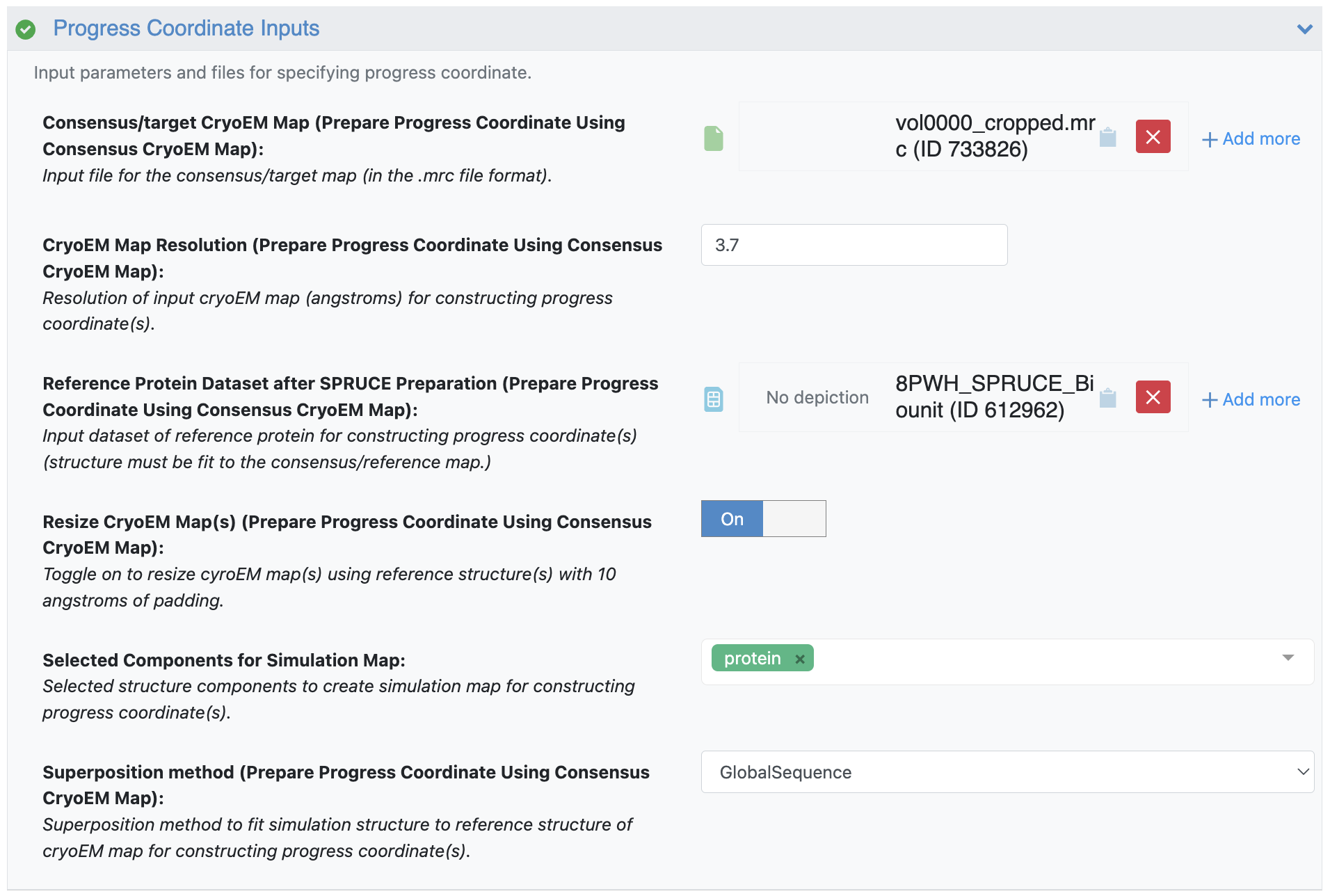
Figure 10. The Progress Coordinate Inputs, showing a specification of 3.7 Å and the k-means cluster center volume 0 (vol0000_cropped.mrc) as the consensus/target cryo-EM map, which will be used in the computation of the RSCC progress coordinate.
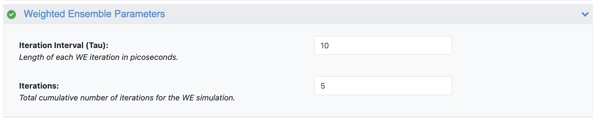
Figure 11. The Weighted Ensemble parameters showing a 5-iteration simulation at 10 ps per iteration.
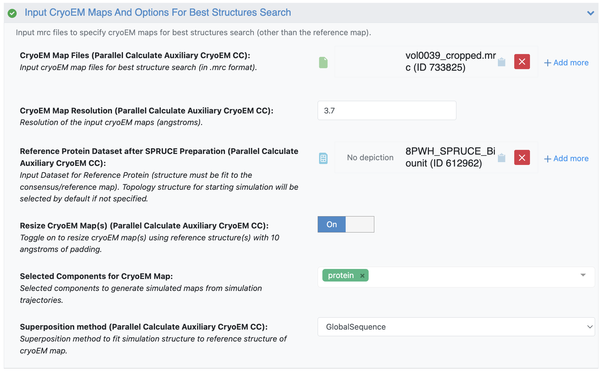
Figure 12. The k-means cluster center volumes 0 and 39 (vol000_cropped.mrc and vol0039_cropped.mrc) maps are provided as the Cryo-EM Map Files target maps for the Best Structures Search parameters. The floe will output a dataset with the structures most consistent with these maps. Two maps have been chosen here, but the floe will output the structures from simulations most consistent with any number of maps.
Note
The Automated WEMD Simulation and Best Structure Search Guided by Target Cryo-EM Map Floe should take approximately 75 minutes to run and cost about $20.
Two Floe Reports are outputted by this floe.
Cryo-EM Map Match Report
The Cryo-EM Map Match Report shows the probability distribution over RSCC values for each map you provided for the Cryo-EM Map Files in the Input Cryo-EM Maps and Options for Best Structure Search parameter group. These probability distributions allow for the estimation of free energy landscapes as a function of the RSCC values as well. In this case, this Floe Report also shows the free energy landscape over both RSCC values, with the RSCC of the first map on the x-axis and the RSCC of the second map on the y-axis. As you only ran five iterations, this free energy landscape should be relatively sparse and flat; longer runs will have more detailed landscapes.
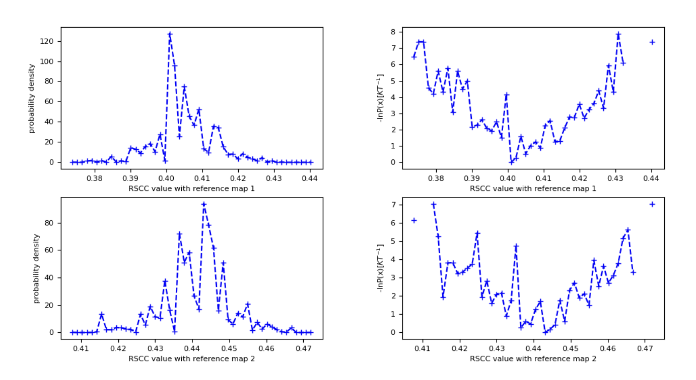
Figure 13. The probability density and free energy plots associated with both maps (vol0000_cropped.mrc and vol0039.mrc).
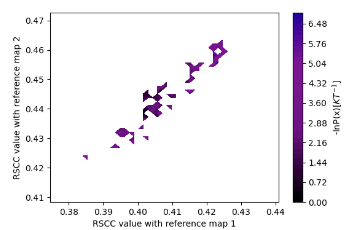
Figure 14. The estimated free energy landscape associated with both maps (vol0000_cropped.mrc and vol0009.mrc), with the RSCC to map 1 along the x-axis and map 2 along the y-axis.
These results show that the simulation generally sampled structures more consistently with map 2 (vol0039_cropped.mrc) than map 1 (vol0000_cropped.mrc), as the probability density has more mass at higher RSCC values.
Start WEMD Simulation and Structure Search Report
This report shows the evolution of the progress coordinate over the WEMD iterations, with the iteration number increasing along the positive y-axis; the probability density over the progress coordinate, showing which RSCC values were sampled more often; the KL-divergence as a function of the iteration number used to evaluate the convergence of the distribution sampled over the iterations (in a 5-iteration test run, this only has one value); and the estimated free energy curve of the progress coordinate.
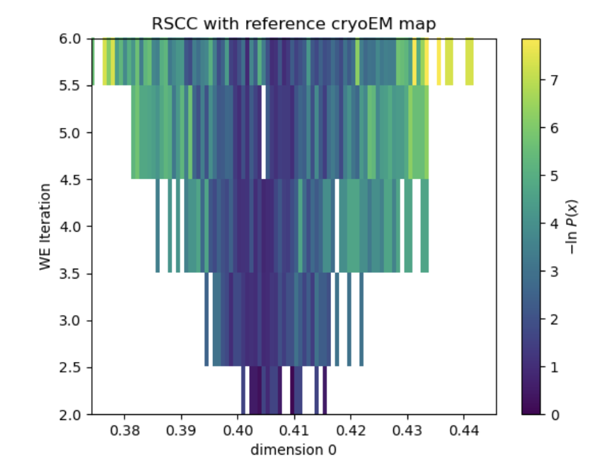
Figure 15. The evolution of the progress coordinate over the 5 iterations of WEMD simulation. The simulation started at an RSCC of about 0.4 and explored RSCC values as high as 0.44.
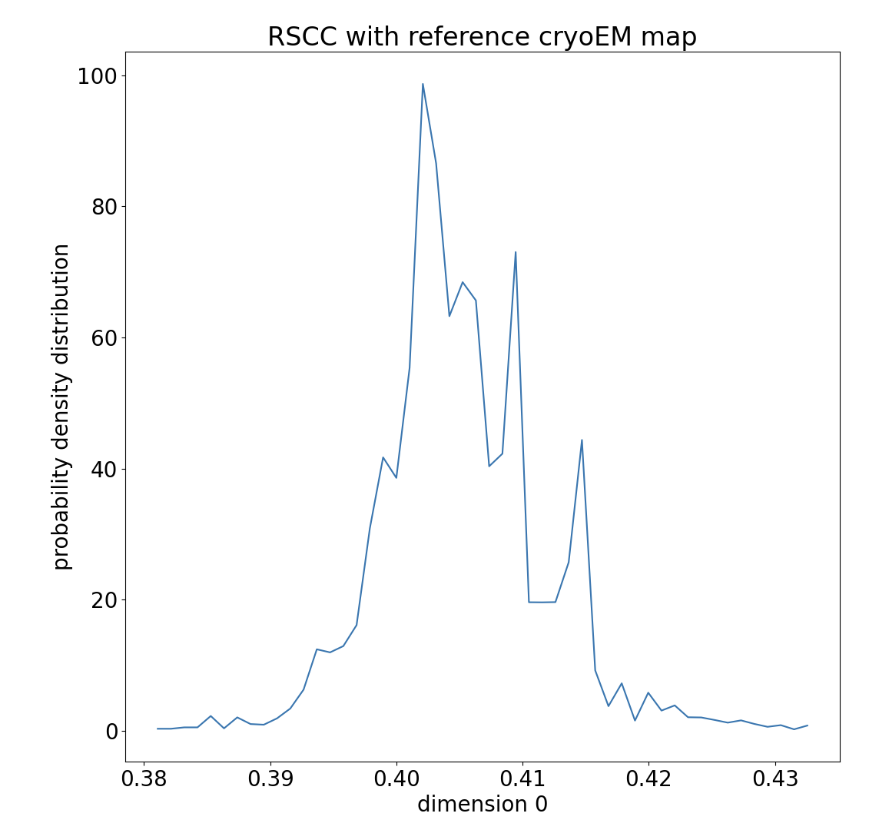
Figure 16. The accumulated probability density distribution over RSCC values sampled in the WEMD simulation.
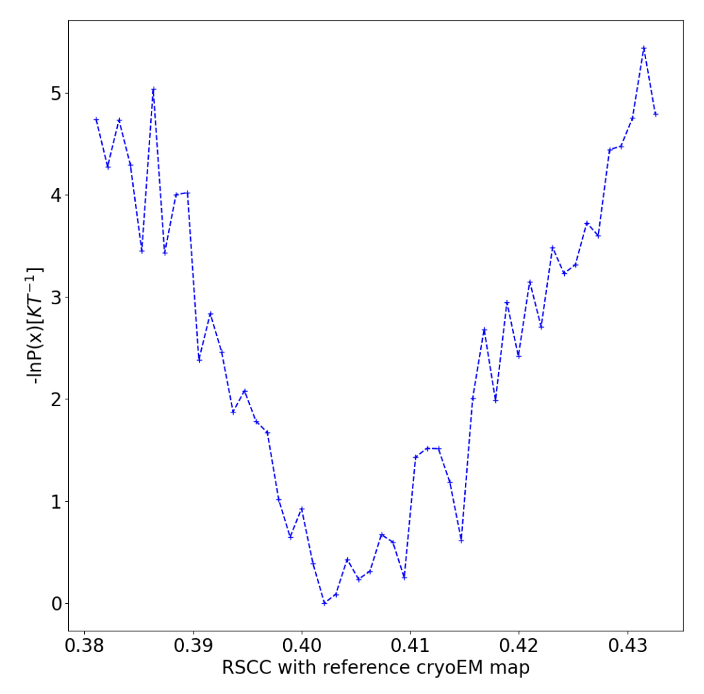
Figure 17. The estimated free energy landscape over RSCC values.
The floe also outputs a best_structure_dataset in the Results section of the Job Details panel. This dataset contains the top five structures from the simulation most consistent with each input map.
To view and analyze the results of the floe in the 3D & Analyze page, follow these steps:
On the Jobs Tab of the Floe page, click the name of the floe job. This will take you to the Job Details Panel.
Under Reports, click the “View in Project Data” button and click the white plus sign next to the dataset. It will become a green checkmark and is now an active dataset.
On the 3D & Analyze page, using the 3D Viewer layout, click the Active Datasets drop-down and toggle on the 3D Only checkmark.
In the data tree under the best_structure_dataset, click the checkmark next to Reference cryo-EM map 0, so it will be visible in the 3D Viewer. Expand the caret and select the “Add new contour” icon (nested circles). Select a color for the map and drag the contour level down to your desired level.
You can view any best_conf_ biounit by clicking the circle next to its name: a green circle means it will be visible.
Expand the caret next to each best_conf_ structure to access the side menu that will allow you to change the color and display style of each bio-unit.
To learn more about the capabilities of the 3D Viewer, please see the documentation for the 3D & Analyze page in the Orion User Guide.
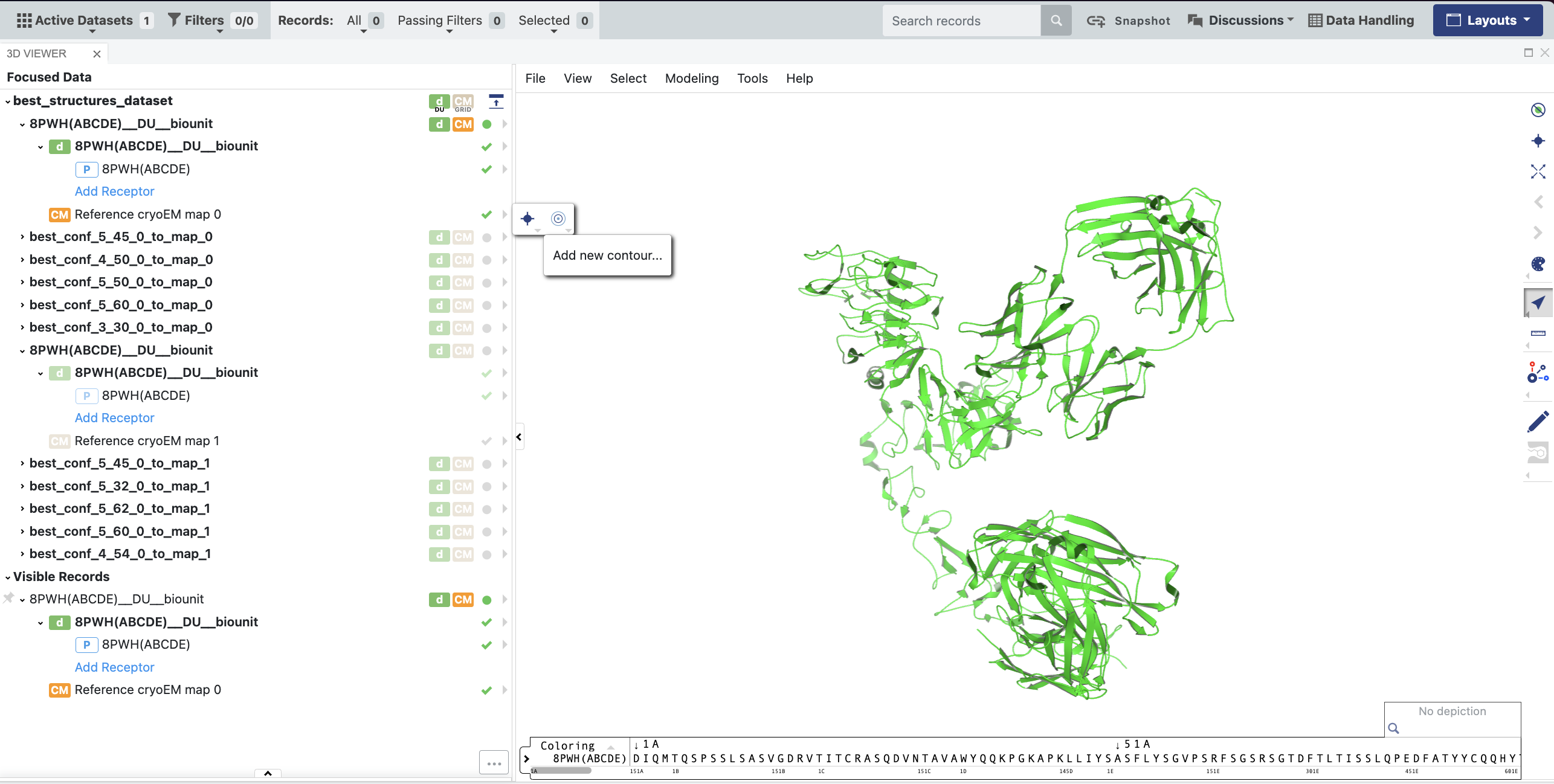
Figure 18. Click the checkmark next to Reference cryo-EM map 0 to make it visible in the 3D Viewer, expand the caret, and click the “Add new contour” icon (nested circles) to adjust the contour level and map color.
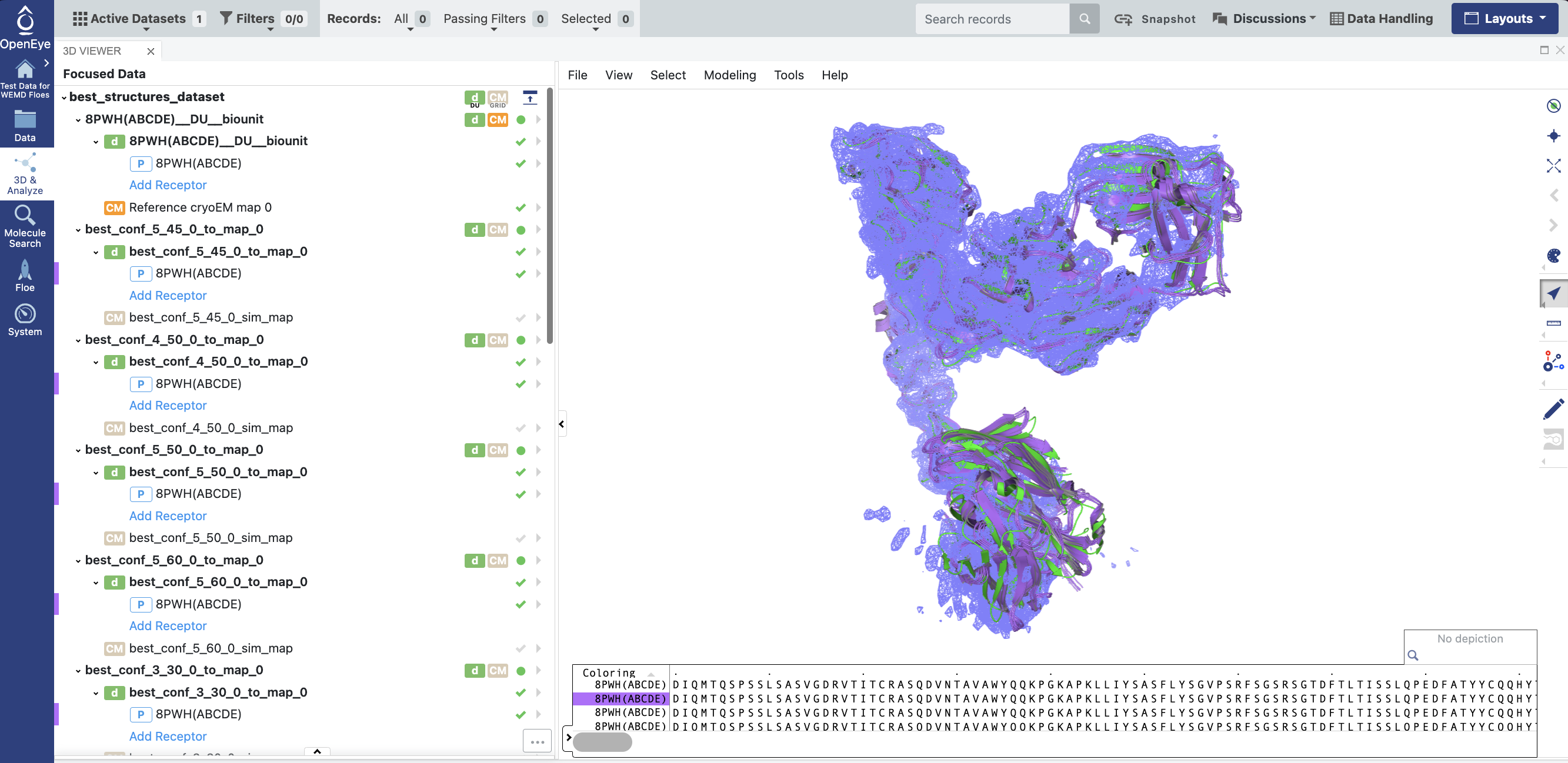
Figure 19. Click the circle next to each Best Structure bio-unit to make it green and expand the caret next to the bio-unit to adjust the color and style of each one.
Simulation Using the Automated Eigenmap Exploration Floe
The Automated WEMD Simulation and Best Structure Search Guided By Eigen CryoEM Maps Floe performs the same best structure search as in the previous floe, but in this case you will use a progress coordinate defined by projecting the heterogeneity onto the eigenmaps from PCA-based particle stack analysis (e.g., RECOVAR or 3DVA). As above, the eigenmaps from the PCA-based particle stack analysis represent the areas of the maps that show the highest variability across the particle stack. For each saved frame of simulation, this floe calculates a simulation map, subtracts the mean map, and performs a regression between the residual map and the eigenmaps, with larger regression coefficients representing higher agreement with the eigenmaps.
Again, it is recommended to start with a short five-iteration test run, to ensure that the results look reasonable before moving to a longer (e.g., 50–100 iterations) simulation using the Continue WEMD Simulation Guided by CryoEM Maps Floe.
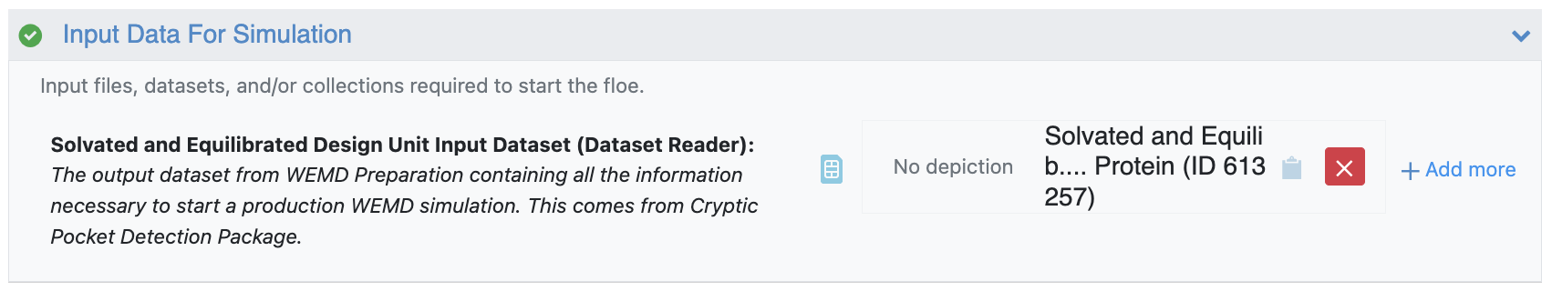
Figure 20. The output dataset from the Solvate and Equilibrate Target Protein Floe is used as the input dataset.
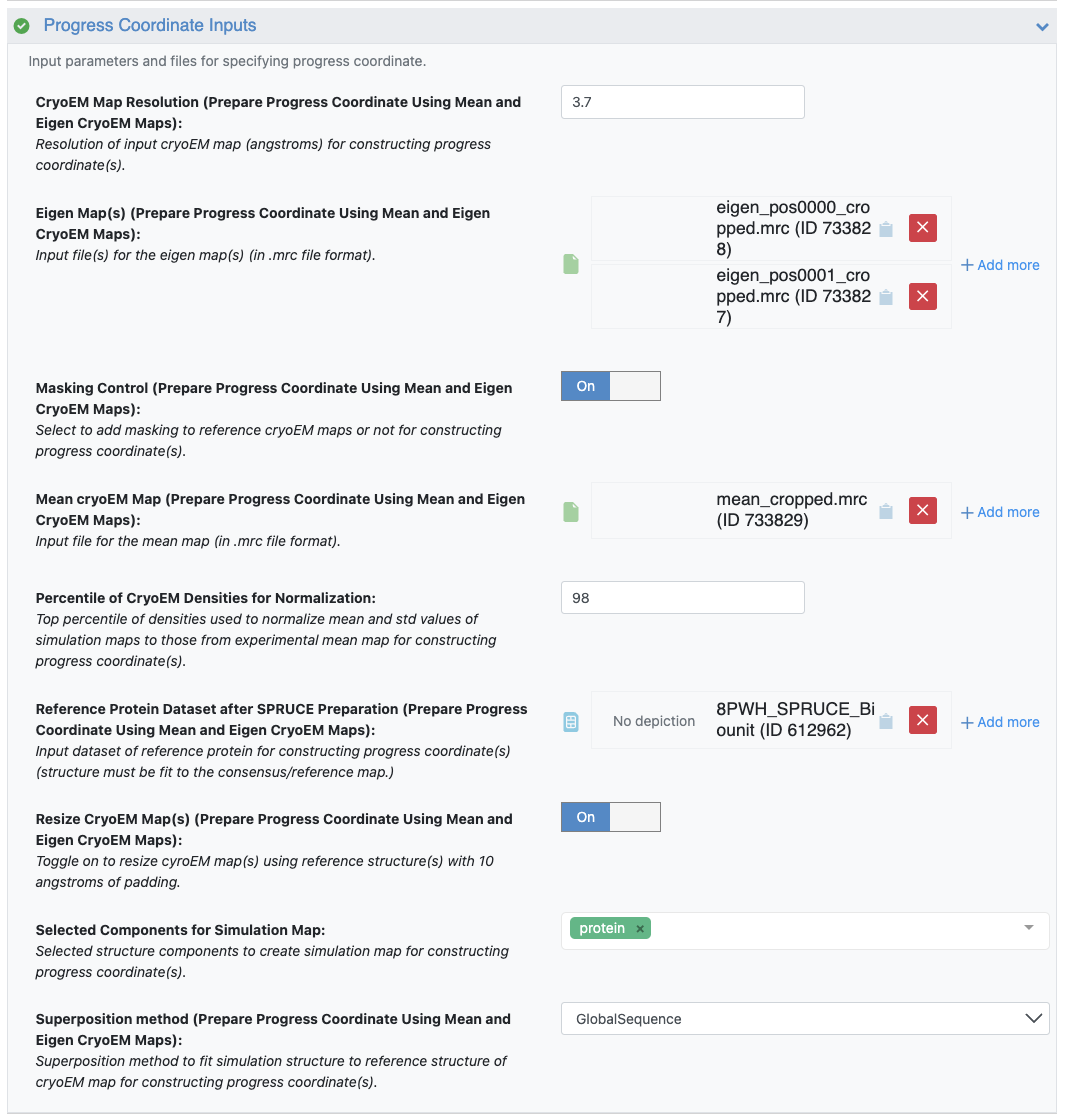
Figure 21. The Progress Coordinate Inputs, specifying Cryo-EM Map Resolution of 3.7 Å, input eigenmaps 0 and 1 (eigen_pos0000_cropped.mrc and eigen_pos0001_cropped.mrc), the mean map (mean_cropped.mrc), and the SPRUCE bio-unit dataset as the Reference Protein Dataset.
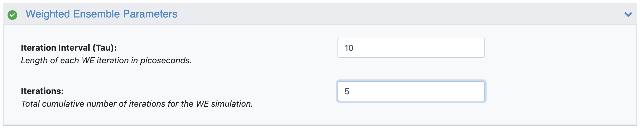
Figure 22. The Weighted Ensemble parameters showing a 5-iteration simulation at 10 ps per iteration.
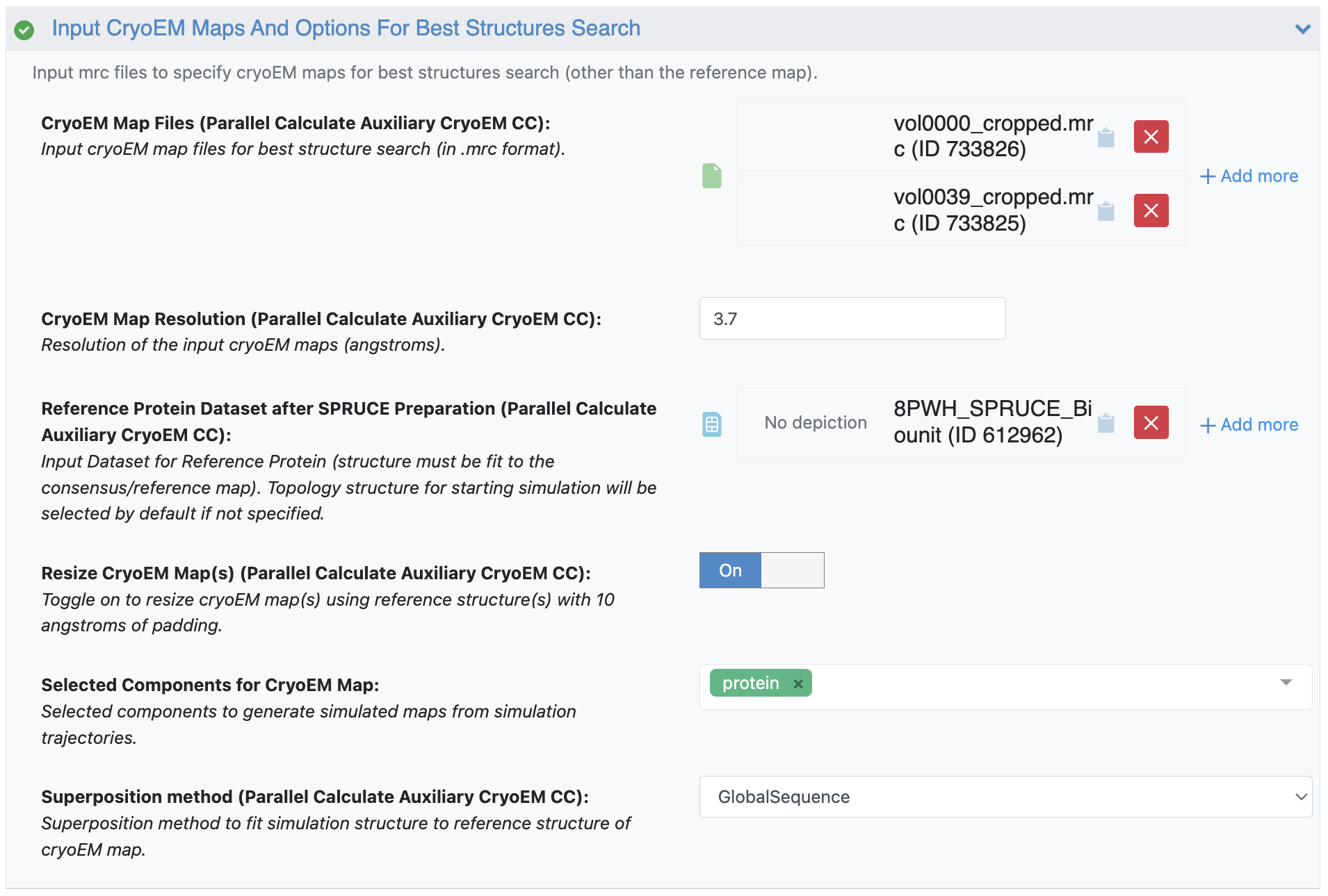
Figure 23. The k-means cluster center maps 0 and 39 (vol000_cropped.mrc and vol0039_cropped.mrc) maps are again used as the Cryo-EM Map Files target maps for the Best Structures Search parameters, with a resolution of 3.7 Å and the SPRUCE bio-unit dataset as the Reference Protein Dataset.
Note
The Automated WEMD Simulation and Best Structure Search Guided By Eigen CryoEM Maps Floe should take approximately 3 hours to run and cost about $60.
Two Floe Reports are outputted by this floe.
Cryo-EM Map Match Report
This report shows the probability distribution over RSCC values for each map you provided for the Cryo-EM Map Files in the Input Cryo-EM Maps and Options for Best Structure Search parameter group. These probability distributions provide an estimation of free energy landscapes as a function of the RSCC values as well. This Floe Report also shows the free energy landscape over both RSCC values, with the RSCC of the first map on the x-axis and the RSCC of the second map on the y-axis. For five iterations, this free energy landscape is relatively sparse and flat; longer runs will have more detailed landscapes.
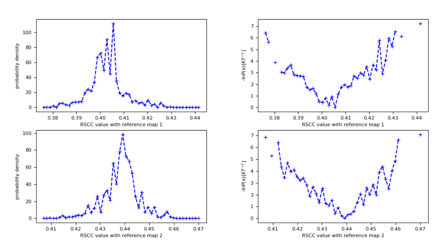
Figure 24. The probability density and free energy plots associated with the input maps (vol0000_cropped.mrc and vol0039.mrc) for the best structure search.
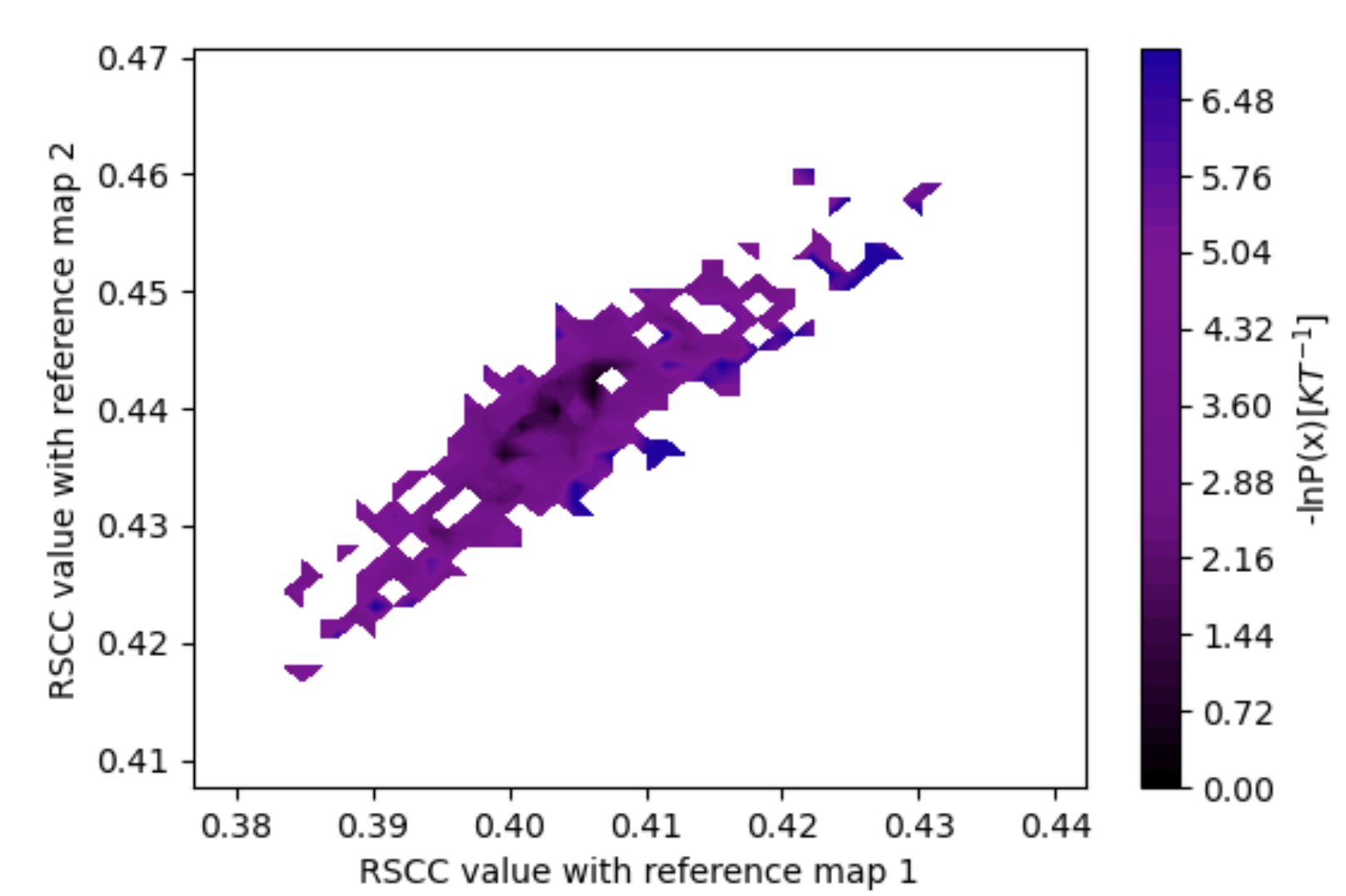
Figure 25. The estimated free energy landscape associated with both maps (vol0000_cropped.mrc and vol0009.mrc) inputted for Best Structure Search, with the RSCC to map 1 along the x-axis and map 2 along the y-axis.
Start WEMD Simulation and Structure Search Report
This report shows the evolution of the progress coordinate over the WEMD iterations, with the iteration number increasing along the positive y-axis; the probability density over the progress coordinate, showing which RSCC values were sampled more often; the KL-divergence as a function of the iteration number used to evaluate the convergence of the distribution sampled over the iterations (in a 5-iteration test run, this only has one value); and the estimated free energy curve of the progress coordinate.
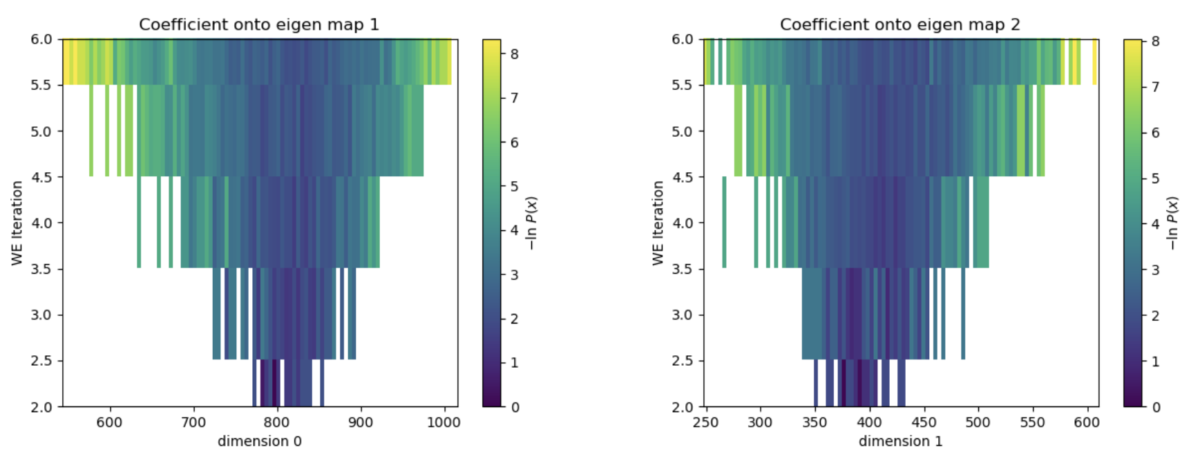
Figure 26. The evolution of the progress coordinate over the five iterations of WEMD simulation. The simulation started at a projection coefficient of about 800 for eigenmap 0 and 400 for eigenmap 1 and explored projection coefficients as high as 1000 for eigenmap 1 and 600 for eigenmap 2.
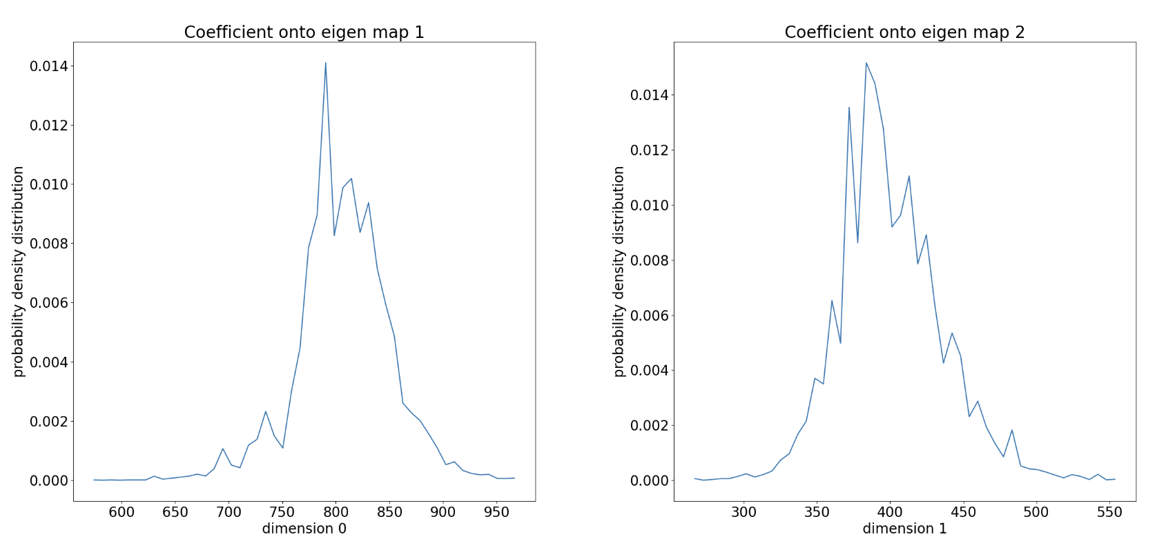
Figure 27. The accumulated probability density distribution over RSCC values sampled in the WEMD simulation.
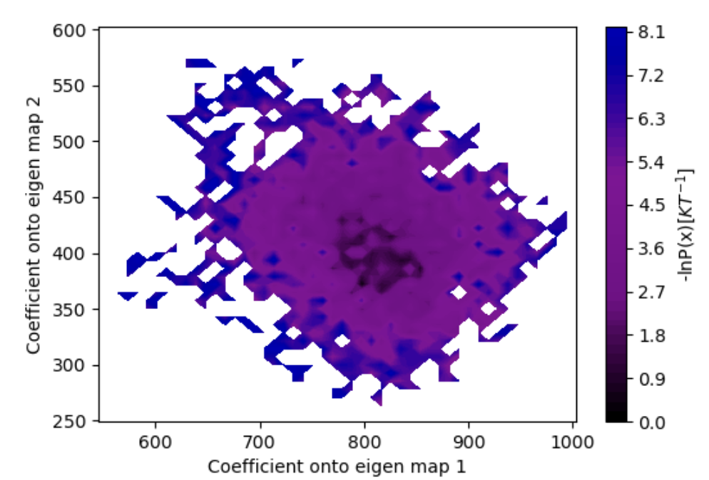
Figure 28. The estimated free energy landscape over projection coefficient values.
You may notice that the coefficients on eigenmaps 1 and 2 are large positive values. This is to be expected. The mean map and the eigenmaps were shown above. The eigenmaps were contoured at values on the order of 1E-7. During a simulation, when you subtract the mean map and find the regression coefficient between the residual map and the eigenmaps, the regression coefficient will be large because the eigenmap values are so small. What is important is the difference in projection coefficient between the two eigenmaps. In this case, the the projection coefficient for map 1 is higher than that for map 2, indicating that the heterogeneity you sampled is more consistent with eigenmap 1 than eigenmap 2.
As with the Automated WEMD Simulation and Best Structure Search Guided by Target Cryo-EM Map Floe, you can examine the best structures for each map by viewing the best_structure_dataset in the 3D & Analyze page. For instructions to view and analyze the results, please see this section.
What to Expect in Longer Runs
In the tutorials for the automated floes above, short five-iteration simulations were used to ensure reasonable results before using the Continue WEMD Simulation Guided by CryoEM Maps Floe to run longer production simulations. This floe uses the wemd_simulation_collection from one of the Automated WEMD Simulation and Best Structure Search Floes as input, as well as the desired total cumulative number of iterations.
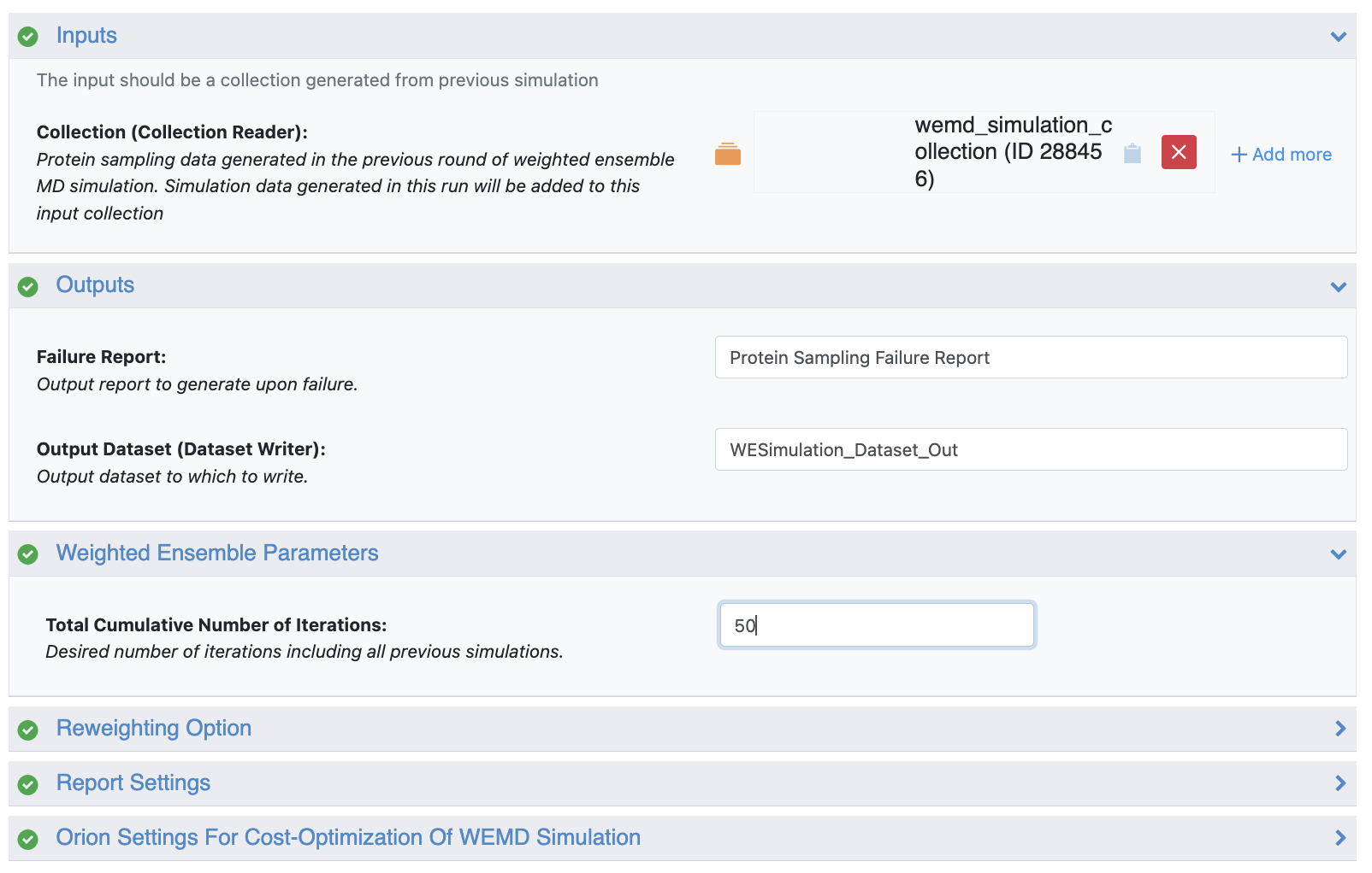
Figure 29. The wemd_simulation_collection from one of the Automated WEMD Simulation and Best Structure Search Floes is used as input and 50 total iterations are selected for our production simulation.
As an example, if the Automated WEMD Simulation and Best Structure Search Guided By Eigen CryoEM Maps Floe simulation is extended to 50 iterations, Figures 30 through 34 are expected in the Floe Report page.
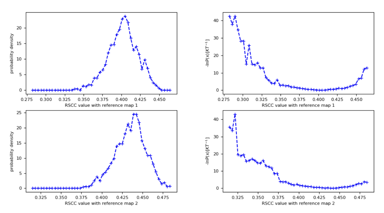
Figure 30. The probability density and free energy plots associated with both input maps (vol0000_cropped.mrc and vol0039.mrc) for the best structure search, extended to 50 iterations. The probability density distributions and free energy surfaces have converged more than the five-iteration example in Figure 24.
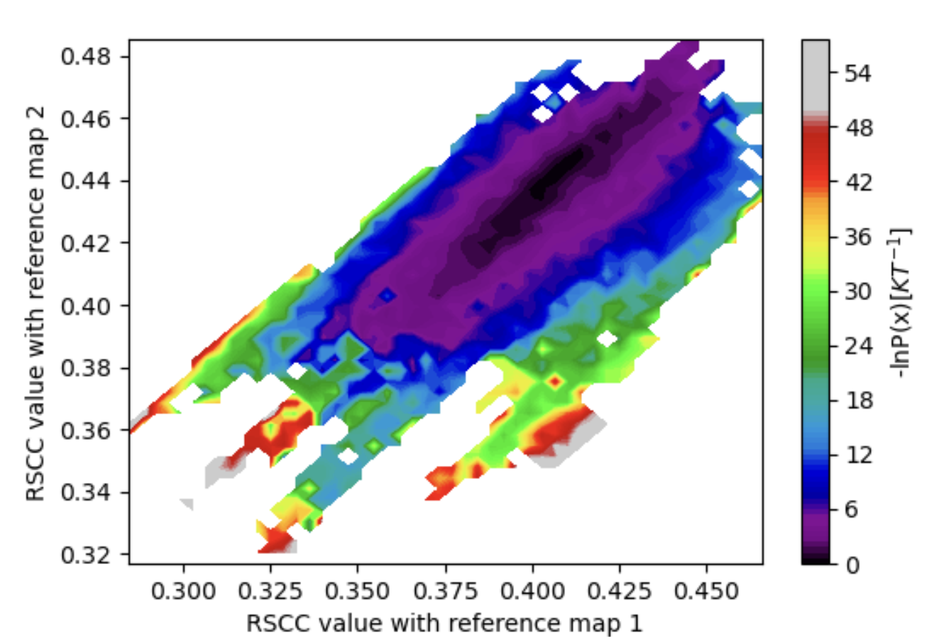
Figure 31. The estimated free energy landscape associated with both input maps (vol0000_cropped.mrc and vol0009.mrc) for the best structure search, with the RSCC to map 1 along the x-axis and map 2 along the y-axis. More iterations allowed exploration of rarer states that are significantly more correlated with map 1 than map 2 and vice versa.
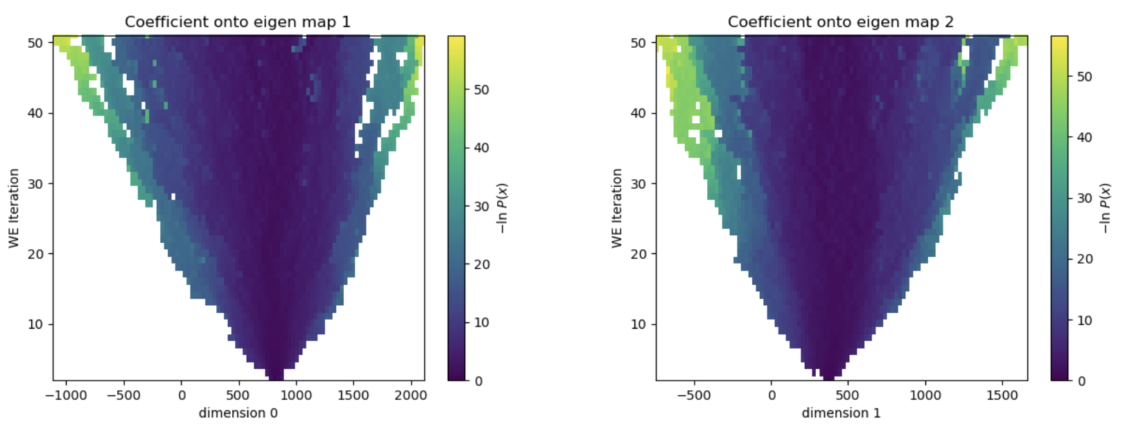
Figure 32. The evolution of the progress coordinate over the 50 iterations of WEMD simulation. The simulation has now explored projection coefficients both very positive and very negative for both eigenmaps 0 and 1.
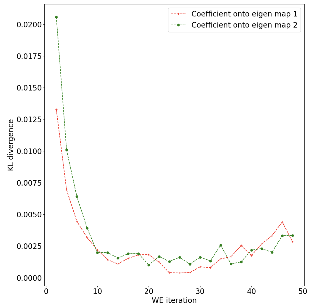
Figure 33. The KL divergence as a function of WEMD iterations. Lower values as the simulation progresses indicate convergence of the probability distribution over progress coordinate values, though the rise in the KL divergence toward the end for map 1 might indicate that further simulation could be beneficial.
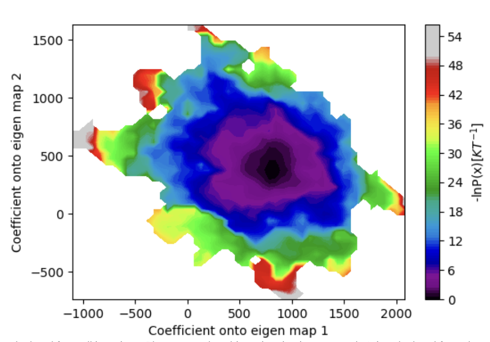
Figure 34. The estimated free energy landscape over the projection coefficient values after 50 iterations.
Note
Fifty iterations of the Automated WEMD Simulation and Best Structure Search Guided By Eigen Cryo-EM Maps Floe should take approximately 30 hours to run and cost up to $800.
Generating the Most Probable Paths Through the Free Energy Landscape
These weighted ensemble simulations send out many walkers during each iteration of simulation, exploring farther reaches of progress coordinate space and accumulating probability weight in regions that are favored by force fields. You can use these walkers to trace a path from the starting point of simulation to regions of interest in the free energy landscape. Walkers are described in more detail in the Generate the Most Probable Path from a WEMD Simulation tutorial.
In the 50-iteration free energy landscape of the Automated WEMD Simulation and Best Structure Search Guided By Eigen CryoEM Maps Floe above, there are a few small free energy basins in regions with higher projections coefficients onto eigenmaps 0 or 1. You can use the Generate Most Probable Path from WEMD Simulation Floe to produce a path from the starting structure to any section of the free energy landscape.
For this example, this floe is used to produce a path from the starting structure to a structure more consistent with eigenmap 1 than eigenmap 0.
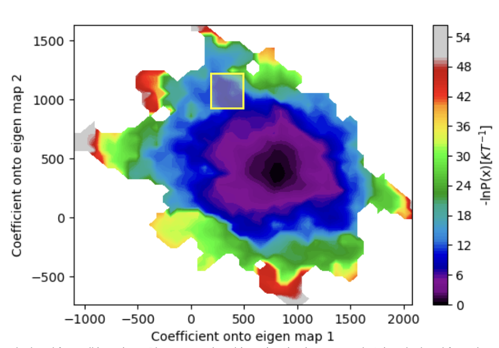
Figure 35. The estimated free energy landscape over projection coefficient values after 50 iterations. The region of interest for path generation is highlighted in the yellow box.
This floe takes as input the simulation collection from the extended simulation, a reference cryo-EM map, a reference protein dataset, and the resolution of the map. It also requires the minimum and maximum bounding box edges for the region of progress coordinate space for the area desired to be the end of the most probable path. Note that you should not select a bounding box that is too small, as the floe may fail if that specific region of progress coordinate space is not sampled in simulation.
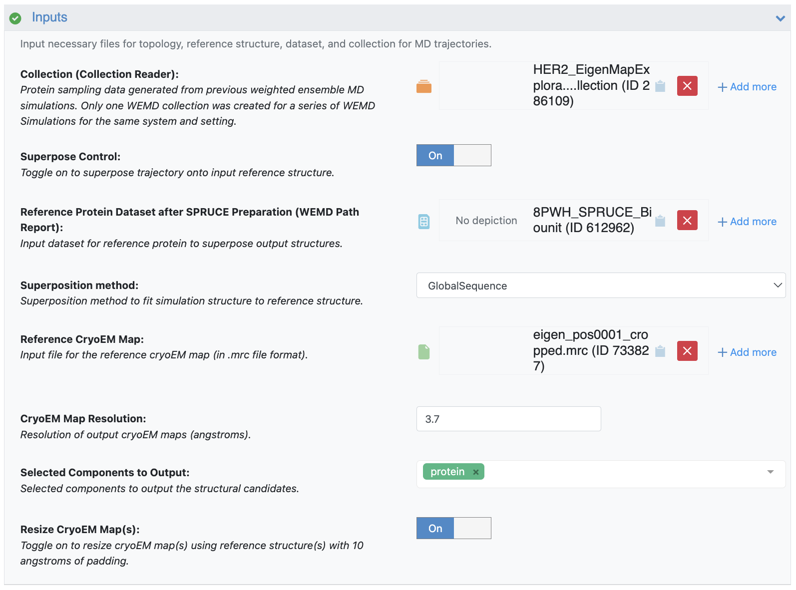
Figure 36. The Job Form showing the inputs of the collection from the extended simulation, the SPRUCE-prepared dataset as the Reference Protein Dataset, the eigenmap 1 mrc file as the reference cryo-EM map, and a resolution of 3.7 Å.
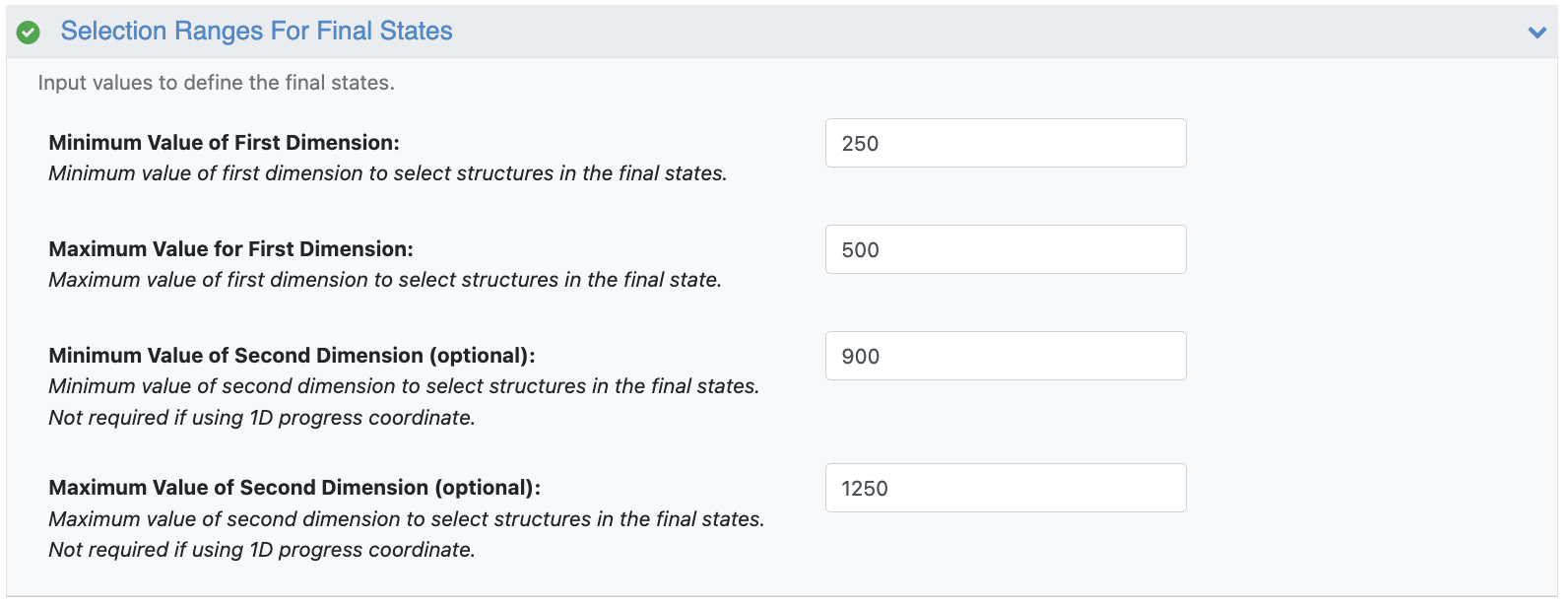
Figure 37. The lower and upper bounds along each progress coordinate axis for the highlighted box in Figure 35.
The floe outputs a path_structures_dataset with a default of 250 samples along the trajectory and a Floe Report showing the path from the starting structure to the region of progress coordinate space selected.

Figure 38. The most probable path from the starting structure to the selected region of progress coordinate space.
Note
The Generate Most Probable Path from WEMD Simulation Floe takes approximately 30 minutes and less than a dollar to run.
The reference cryo-EM map can be loaded into the 3D viewer and compared with structures that represent samples from along the most probable path from the starting structure to the region of progress coordinate space specified on the Job Form. Figure 39 shows an example using eigen_pos0001_cropped.mrc as the reference cryo-EM map, compared to the final structure from the most probable path trajectory (frame 250).
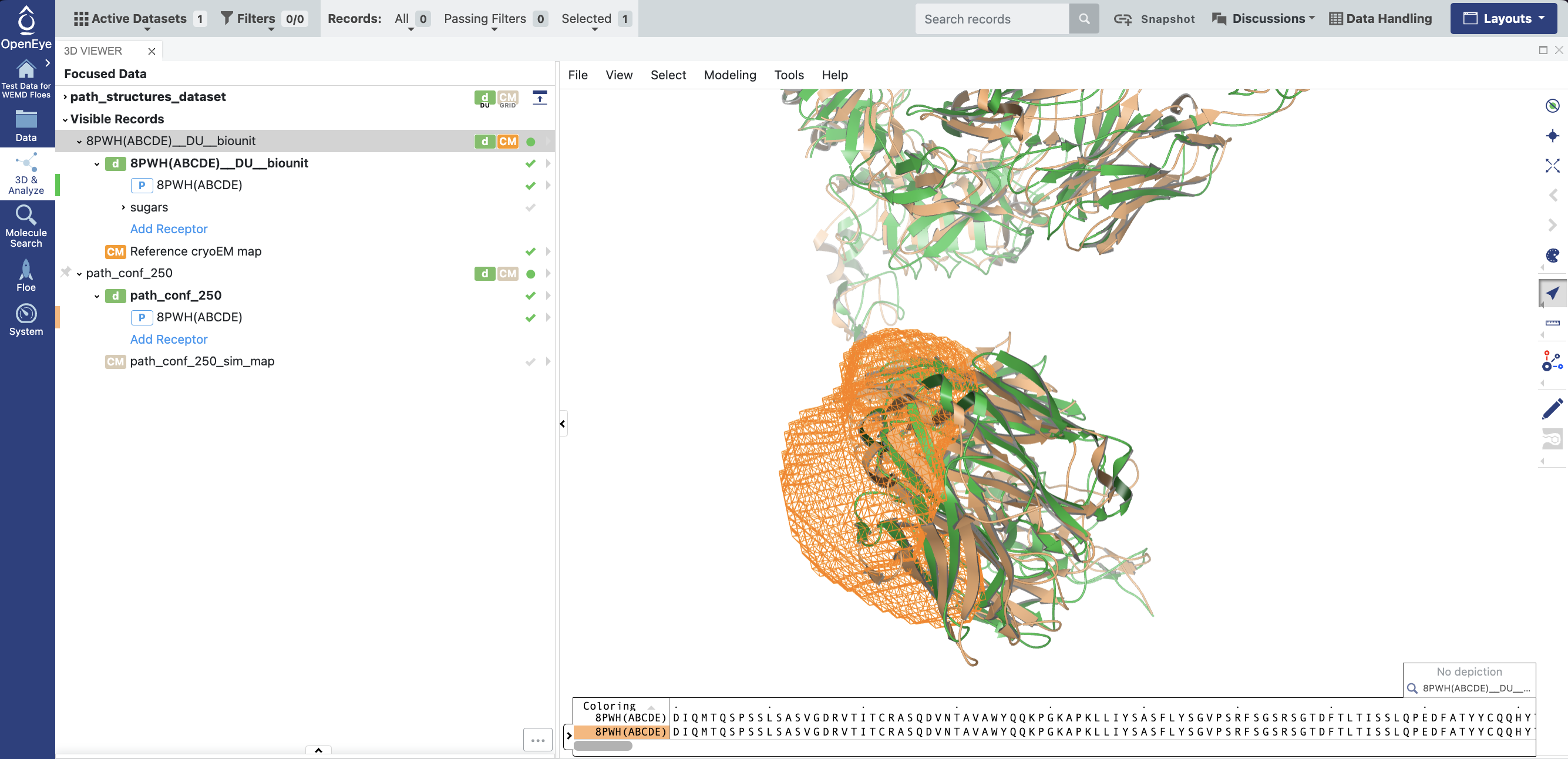
Figure 39. Eigenmap 1 (orange mesh), the reference bio-unit from SPRUCE (green cartoon protein visualization) and the final structure from the most probable path trajectory (orange cartoon protein visualization). The traztuzumab region has shifted to toward the eigenmap region.
Identifying Pockets From the Simulation
The simulation collections can be used as input to the Cryptic Pocket Detection Floes to identify cryptic pockets that have opened over the course of a simulation.
In this example, use the Probe Occupancy Analysis Floe, which requires only the simulation collection as input: specifically, the 50-iteration Eigenmap Exploration Collection. This floe will analyze the occupancy of the xenon atom probes around the protein to identify pockets suitable for downstream analysis.
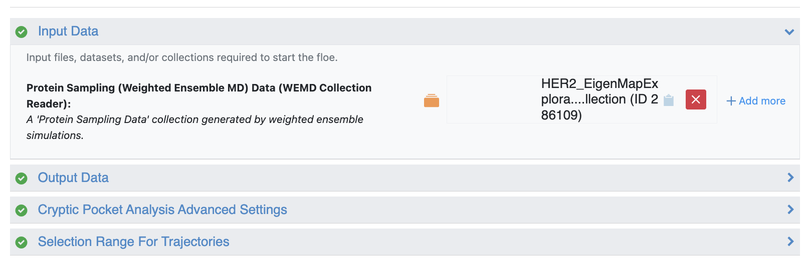
Figure 40. The Probe Occupancy Analysis Floe requires only the simulation collection from the 50-iteration Generate Most Probable Path from WEMD Simulation Floe as input.
Note
The Floe Report pages for Cryptic Pocket Analysis Floes can be quite large, so they may require a long time to load.
The Cryptic Pocket Detection Analysis Floes output a Floe Report containing the ranked network of pockets that were detected in simulation and related by edges corresponding to their interpocket center of mass distance.
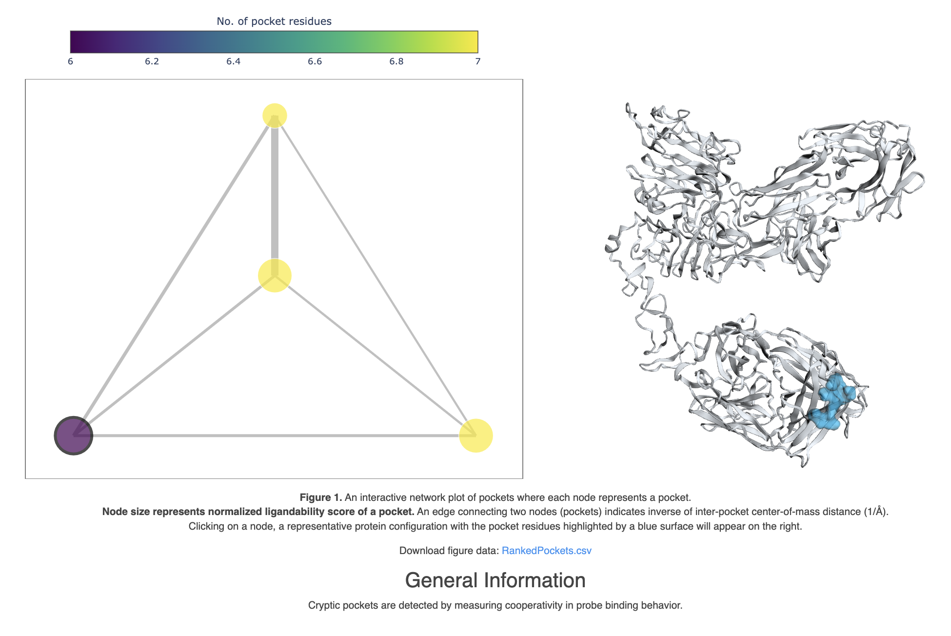
Figure 41. The Probe Occupancy Analysis Floe Report shows the highest ranked pocket on the traztuzumab chain.