ML Build: Classification Model with Tuner using Fingerprints for Small Molecules

In this tutorial, we will train several classification models to predict IC50 concentrations at which molecules become reactant to pyrrolamides. The IC50 responses are divided into Low, Medium, and High based on a quartile based cutoff. The training data is known as the PyrrolamidesA dataset. The classification models will be built on a combination of fingerprint and neural network hyperparameters. The results will be visualized in both the Analyze page and the Floe Report. We will use the Floe Report to analyze and choose a good model. Finally, we will choose a built model to predict the properties of some unseen molecules.

This tutorial uses the following floe:

• ML Build: Classification Model with Tuner using Fingerprints for Small Molecules

Warning

This tutorial keeps default parameters and builds approximately 1K machine learning models. While the per model cost is very cheap based on the size of dataset, the total cost might be expensive. For instance, with the pyrrolamides dataset (~1K molecules), it costs around $100. To understand the working of the floe, we suggest building lesser models by referring to the Cheaper and Faster Version of the tutorial. This option builds regression models, but the idea to reduce parameters should hold for classification as well.

Note

If you need to create a tutorial project, please see the Setup Directions for the Machine Learning Model Building Tutorials.

Floe Input

This floe uses the PyrrolamidesA dataset for P₁. The floe expects two things from each record:

• An OEMol, which is the molecule to train the models on.

• A String value that contains the classification property to be learned. For this example, it is the Low, Medium, or High IC Class of the NegIC50 concentration.

Here is a sample record from the dataset:

OERecord (
    *Molecule(Chem.Mol)* : c1cc(c(nc1)N2CCC(CC2)NC(=O)c3cc(c([nH]3)Cl)Cl)[N+](=O)[O-]
    *IC Class(String)* : Low
)

Input Data

PyrrolamidesA dataset

Run OEModel Building Floe

Choose the ML Build: Classification Model with Tuner using Fingerprints for Small Molecules Floe. Click “Launch Floe” to bring up the Job Form. The parameters can be specified as below.

• Input Small Molecules to Train Machine Learning Models On: Select the PyrrolamidesA dataset or your own dataset.

• Outputs parameter: You can change the names of the built ML models to be saved in Orion, but we will use the defaults for this tutorial.

• Response Value Field: This is the property to be trained. The drop-down field generates a list of string options based on the input dataset. For our data, it is IC Class.

• Are We Using Keras Tuner: This indicates whether to use a hyperparameter optimizer with a Keras tuner. Keep this On by default.

• What Kind of Keras Tuner to Use: Keep Hyperband as the default or change to another option.

• Number of models to show in Floe Report: This field prevents memory blowup in case you generate >1K models. In such cases, viewing the top 20–50 models should suffice.

The input molecules and the training field values can be filtered and transformed by preprocessing.

• Preprocess Molecule performs the following steps:

  • Keeps the largest molecule if more than one is present in a record.

  • Sets the pH value to neutral.

• If you don’t preprocess the molecule, you can still apply the Blockbuster Filter if needed.

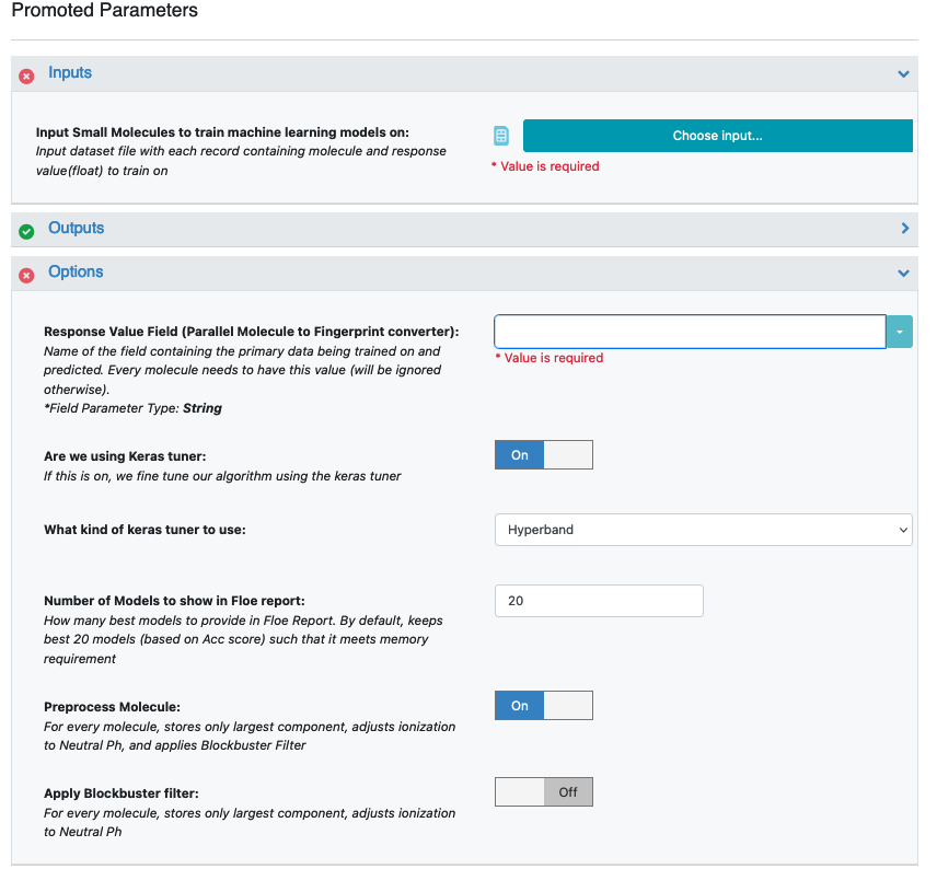
Figure 1. Options parameters on the Job Form.

• The default parameters create a working model. But we can tweak some parameters to learn more about the functionalities.

Advanced: Cheminformatics Fingerprint Options: These parameters contain the cheminformatics information the model will be built on. We can change or add more values to the fingerprint parameters as shown below.

• For suggestions on tweaking, read the How-to-Guide on building Optimal Models.

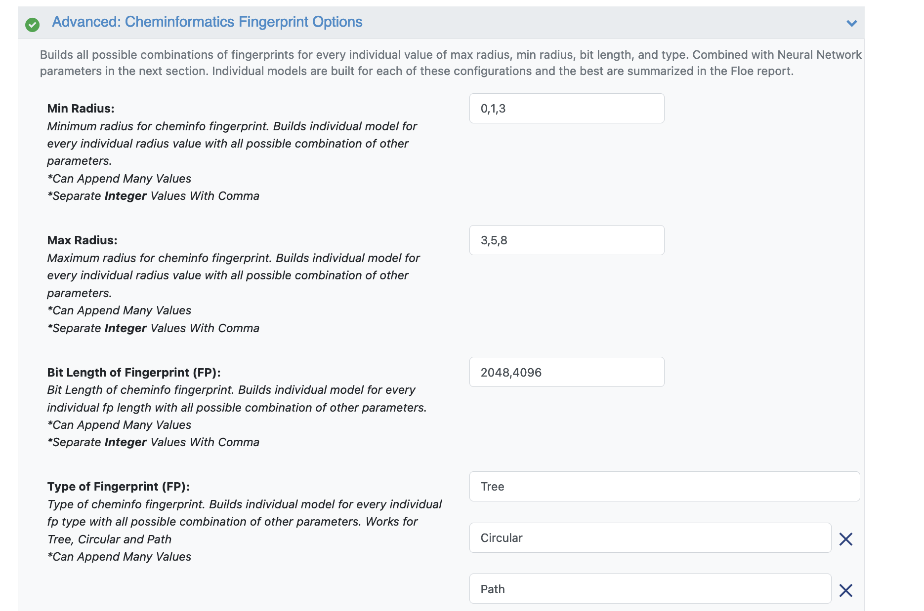
Figure 2. Parameter options for cheminformatics fingerprints.

Advanced: Neural Network Hyperparameters Options: These are more specific machine learning parameters. Again, we can use the defaults or choose to add or modify some values based guidance from the How-To Guide.

• Dropouts: These can be added to prevent overfitting.

• Sets of Hidden Layers: Every row is the node size of each layer.

  • Since it is a -1 separated list, by default there are 3-layer networks of size (250,150,50) and (150,100,80).

  • This gives a total node size of 330(150+100+80) and 240(100+80+60) in the default models.

  • Plugging in the formula stated in the How-to-Guide building Optimal Models, we should reduce the number of nodes to prevent overfitting.

  Note that there is a bug in the current description of this parameter. It should read the following: “Eg: by default each lists first tuple will create NN with 3 hidden layers of size 10,25,50. (Vertically pick first value of each row). Followed by 10,25,75 (row1col1, row2col1, row3col2) | 10,25,100 (row1col1, row2col1, row3col3)| 10,50,50 (row1col1, row2col2, row3col1)”

• Sets of regularization layers: This field sets L2 regularization for each network layer, making it a -1 separated 3-tuple list as well. Note that the current defaults are 0.04,0.02 and 0.02,0.01,0.01. There is a bug in this parameter description as well.

• Learning Rate: Increasing this parameter speeds things up, although the algorithm may not detect the minima if this value is too high. We can train our model on multiple learning rate values. Use the default values for this tutorial.

• Max Epochs: If the dataset is big, consider increasing the epoch size, as it may take the algorithm longer to converge. Use the default values for this tutorial.

• Activation: ReLU is a commonly used activation function for most models. If needed, change this parameter to one of the options in the list (see How-to-Guide on building Optimal Models).

• Batch Size: This defines the number of samples that will be propagated through the network. With larger batches, there is a significant degradation in the quality of the model, as measured by its ability to generalize. However, too small of a batch size may cause the model to take a very long time to converge. For a dataset size of ~2 K, 64 is a reasonable batch size. However, for datasets of approximately 100 K, we may want to increase the batch size to at least 5 K.

• Set the batch size to 64 or keep the Adjust Batch Size* toggle On.

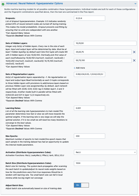
Figure 3. Neural network hyperparameter options.

That’s it! Let’s run the floe. Click the “Start Job” button.

Note

The default memory requirement for each cube has been set to moderate to keep the price low. If you are training larger datasets, be mindful of the time it takes for the cubes to run to completion. Increasing the memory will allow Orion to assign instances with more processing power, thereby resulting in a faster completion. In some cases, the cubes may run out of memory (indicated in the log report) for large datasets. Increasing cube memory will fix this as well.

Analysis of Output and Floe Report

After the floe has finished running, click the link on the Floe Report tab in your window to preview the report. Since the report is big, it may take a while to load. Try refreshing or popping the report out to a new window if this is the case. All results reported in the Floe Report are on the validation data.

Figure 4 shows statistics for all input data. The histograms represent the spread of data for each property of the input molecules. Skewed histograms or outliers may indicate the need for the data preprocessing floe in order to build better models.

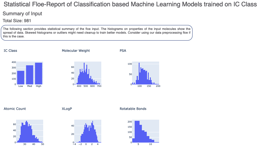
Figure 4. Histograms for the summary statistics of the input data.

The graphs in Figure 5 show the accuracy on the validation set for different values of the cheminformatics and neural network hyperparameters. They indicate how model performance fluctuates with change in a single hyperparameter when all others are kept constant. They help us analyze the sensitivity of different hyperparameter values and plan future model builds accordingly. For instance, the graph below shows that a dropout of 0.1 and maxr of 5 are better choices for these parameters.

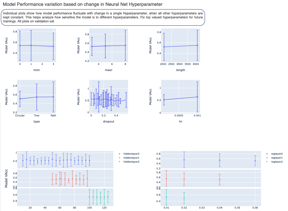
Figure 5. Model performance based on varying the hyperparameters.

There is also a plot between the top two most sensitive hyperparameters.

In the example below, the two most sensitive parameters are regularization 1 and regularization 0. Choosing values around the minima in the MAE heatmap (0 for reglayer1 and 0.04 for reglayer2) will build better models in future attempts.

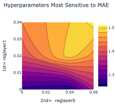
Figure 6. The two most sensitive hyperparameters.

Next, we tabulate a list of all models built by the fully connected network. These models are sorted by their Acc Score. On the face of it, the first row should be the best model since it has the least error on the validation data. But several other factors besides Acc Score influence this, starting with VLoss in the next column. Click on a Model Link to get details on each model built. The best models to use for prediction are those with low overfit correlations and good validation scores.

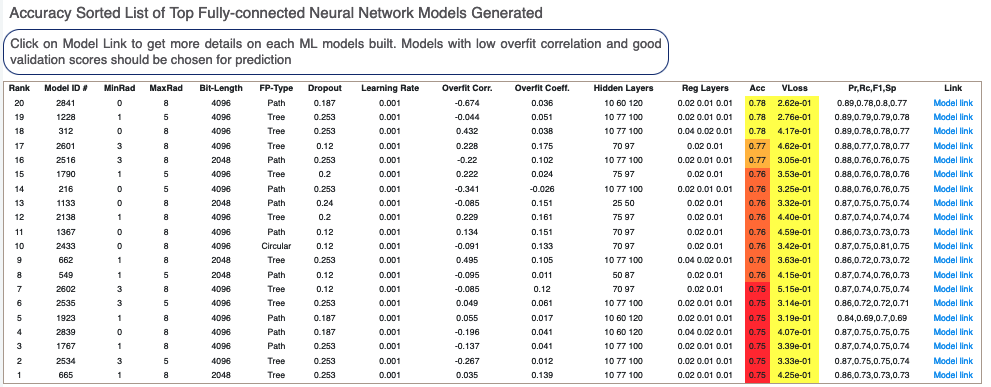
Figure 7. List of generated fully connected neural network models.

For the top-ranked model, there is a linear color scale showing the rank. The cheminformatics and machine learning training parameters are shown below.

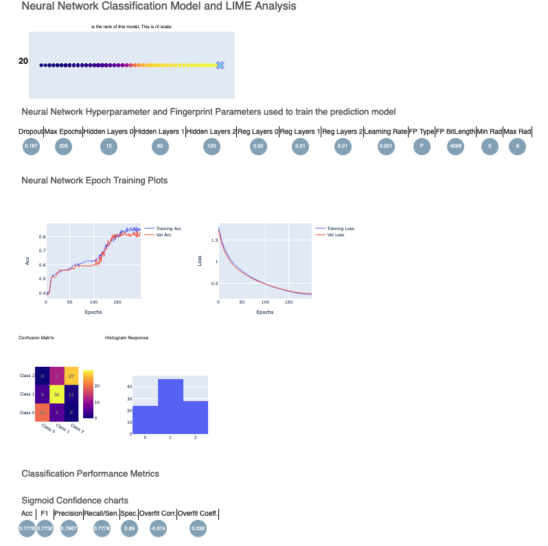
Figure 8. Neural network classification model and LIME analysis.

The Neural Network Epoch Training Plots show the curves for the training and validation Acc and Loss. These curves are relatively close, which indicates an absence of overfitting. Although the confusion matrix and the F1, Precision, and Recall scores are reasonable, it is best to look at other models as well.

In contrast, here are plots for Model Link 5. We see that the training and validation Acc follow a similar trend, which shows a good sign of not overfitting. Had they been diverging, we might need to further tweak parameters such as number of hidden layer nodes, dropouts, regularizers, and so on. Too much fluctuation in the graphs would suggest a slower learning rate. The confusion matrix and performance metrics look reasonable as well, making Model 5 a good candidate to predict the NegIC50 value of unknown molecules.

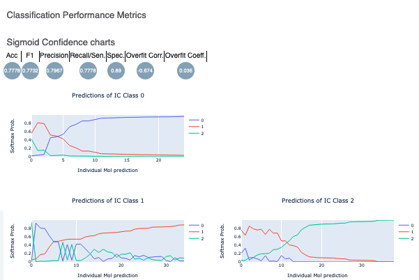
Figure 9. Performance metrics and sigmoid confidence plots for Model Link 5.

Lastly, the Sigmoid Confidence Chart plots show that the final sigmoid layer of the neural network is discernible. As shown in the first graph, the IC Class zero has a greater softmax probability than either 1 or 2. The same holds of the prediction of the other two IC Classes. These plots illustrate that the sigmoid layer is confident in its prediction on the validation data. This is another sign of good model training.

Below that, annotated explainers of the machine learning model are shown. You can click on interesting molecules to see explanations of both correct and incorrect predictions of outliers.

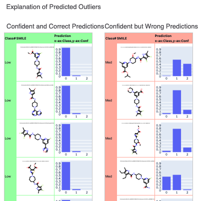
Figure 10. Explanation of predicted outliers.

This tutorial shows how to build classification models; it’s important to remember that building an optimized model is a nontrivial task. Refer to the How-to Guide on building Optimal Models.

After we have found a model choice, we can use it to predict and or validate against unseen molecules. Go to the Use Pretrained Classification Fingerprint Model to Predict Properties of Molecules tutorial to do this.