Short Trajectory MD with Analysis for Pose Validation
The primary purpose of the Short Trajectory MD with Analysis (STMD) Floe is the pose validation. In this tutorial, we will present how we run the Floe and understand the results for pose validation of (1) single ligand with single pose; (2) single ligand with multiple docked poses; and (3) a set of ligands.
Floe Inputs
The ligand input datasets used in this tutorial are:
The protein input dataset used in this tutorial is:
Running Floe
After selecting the Short Trajectory MD with Analysis Floe in the Orion UI, you will be presented with a job form with parameters to select. The parameter to change in this tutorial is:
Bound State Equilibration Production Time (default 6): 2. The default 6 is set to be synchronized with the De Groot protocol, so that the output ligand-bound/unbound datasets can be directly used in nonequilibrium switching Floe. For the pose validation, we set the production time to 2.
Understanding the results for a single ligand
The results from the STMD Floe are accessed via two main avenues: through the job output in the Jobs tab in Orion’s Floe page, and through Orion’s Analyze page. We will look at the results of two jobs run on the same MCL1 ligand; in the first case the input ligand had only a single pose and in the second case it had six slightly different docked poses.
MCL1 ligand 35: single input pose
First we will look at the results of the single-pose run, with default of 1 for Number Of Bound State MD Starts: one start of one ligand with one pose, so one 2 ns MD run overall. In the Jobs tab in Orion’s Floe page, having selected the job name for your STMD job, you should land on the job results page. The left panel contains the usual Orion job information from the run, and the right panel has two tabs at the top once the job has completed successfully. Selecting the second tab called FLOE REPORT should give you a page looking similar to Figure STMD Job results page for a single pose of an MCL1 ligand.
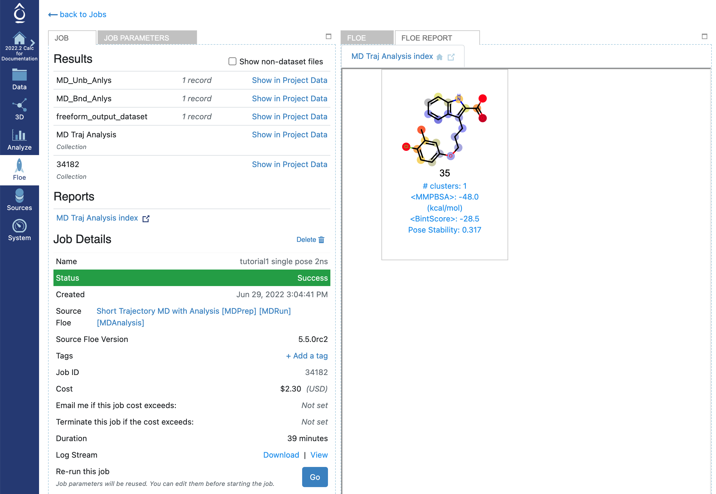
STMD Job results page for a single pose of an MCL1 ligand
The Floe report shows a tile for each MD simulation, here there was only one ligand in the input file. The atom colors correspond to calculated B-factors, similar to Xray B-factors, depicting the mobility of those atoms in the active site over the course of the MD trajectory. This gives an immediate read-out on how much various fragments of the ligand were moving around in the active site. As a general principle greater movement suggests that that fragment is not as tightly bound in the active site, but inferences are only qualitative. Certainly fragments hanging out in water of even a tightly bound inhibitor will be expected to be more mobile than the buried parts. Other information on each tile is:
The ligand name.
The number of clusters formed by clustering the ligand positions in the MD trajectory.
The Boltzmann-weighted MMPBSA score for ligand binding over the trajectories for all poses.
The simple ensemble average BintScore [1] for ligand binding over the trajectories for all poses (lower score is better).
The stability of the pose relative to the starting pose (varies between 0 (no stability) and 1 (completely stable)).
Clicking on the tile drills down into the detailed analysis of that simulation, resulting in Figure Detailed results for ligand 35 (single pose):
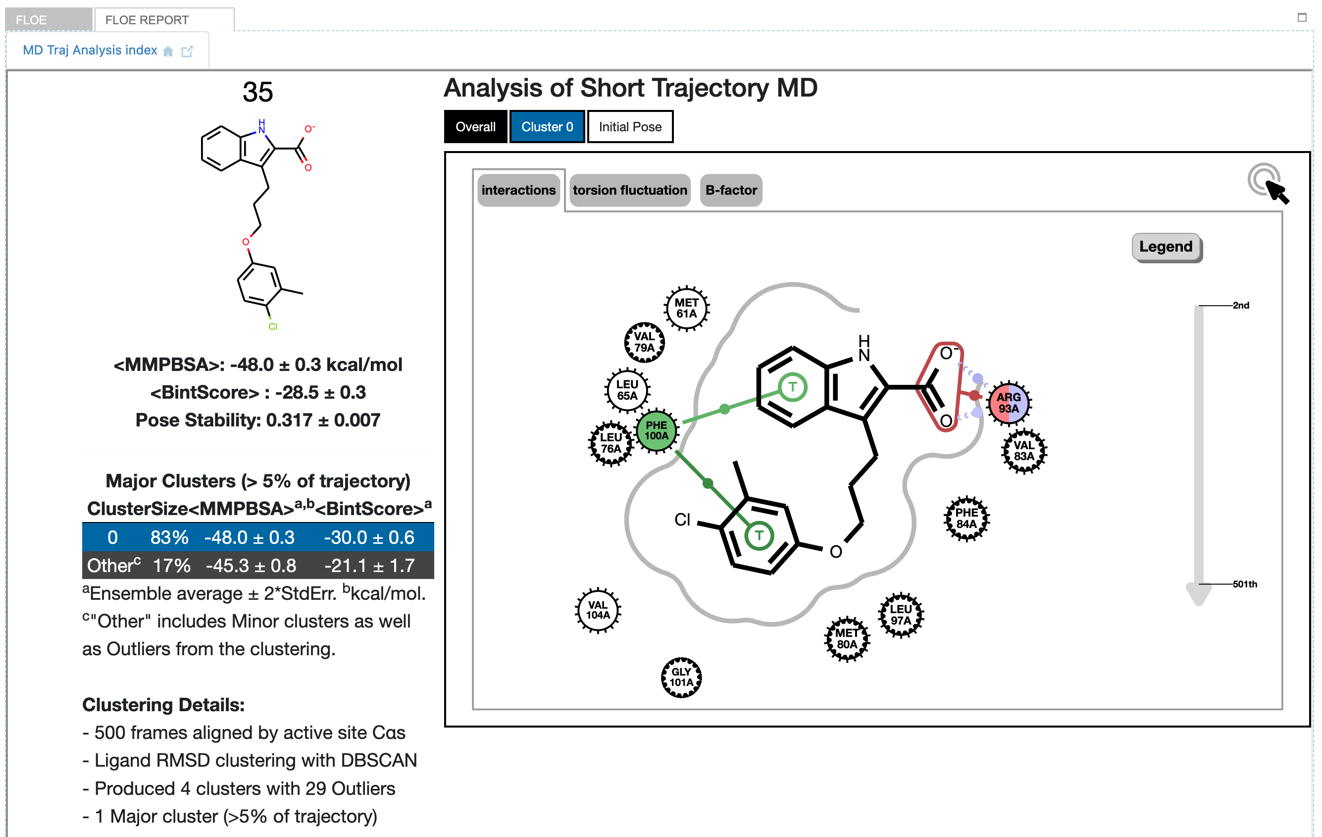
Detailed results for ligand 35 (single pose)
In this MD run, the results show a single cluster for the whole trajectory. Because MD is only sampling an equilibrium, the results are not deterministic: In you run this same MD again, in principle you could get slightly different results. Nevertheless, the results are interpreted in the context of the sampling obtained.
In the graphic we see a 2D representation of the ligand binding interactions for the whole trajectory, with the default display of the Overall tab at the top of the graphic. It is an interactive graphic: selecting the Cluster 0 tab in blue will change the binding interaction representation to that corresponding to the selected cluster. Hovering over one of the interactions in the diagram lights up a strip chart on the right-hand side grey arrow showing the occupancy of that interaction over the course of the trajectory. Within the heavy frame of the graphic, we see that the interactive graph is on interactions; selecting torsions changes the depiction to show a heavy black dot in each rotatable bond. Hovering over one of these shows a radial bar graph of the occupancy of the torsion on the right-hand side. Selecting B-factor yields a depiction of the calculated B-factors for the selected cluster as in the parent tile, but additionally shows the calculated B-factor for each active site amino acid close to the ligand. To the left of the graphic is information about the clustering of the ligand trajectory, including a table giving the ensemble average MMPBSA energy and BintScore (each with standard error) for each cluster. The MMPBSA value represents a Boltzmann-weighted average over all major clusters, but for BintScore it is a simple ensemble average for the ligand as a whole. Note with only one cluster here, the Boltzmann-weighted result represents cluster 0 completely. The remaining value, “Pose Stability”, is derived from the ensemble BintScore and represents how stable the overall protein-ligand binding interactions are compared to the starting pose (varies between 0 (no stability) and 1 (completely stable)).
Scrolling down exposes a strip chart and two tables detailing relevant analyses of the trajectories for all poses of the ligand. The strip chart for ligand 35 (single pose) is shown in Figure Strip Chart results for ligand 35 (single pose):
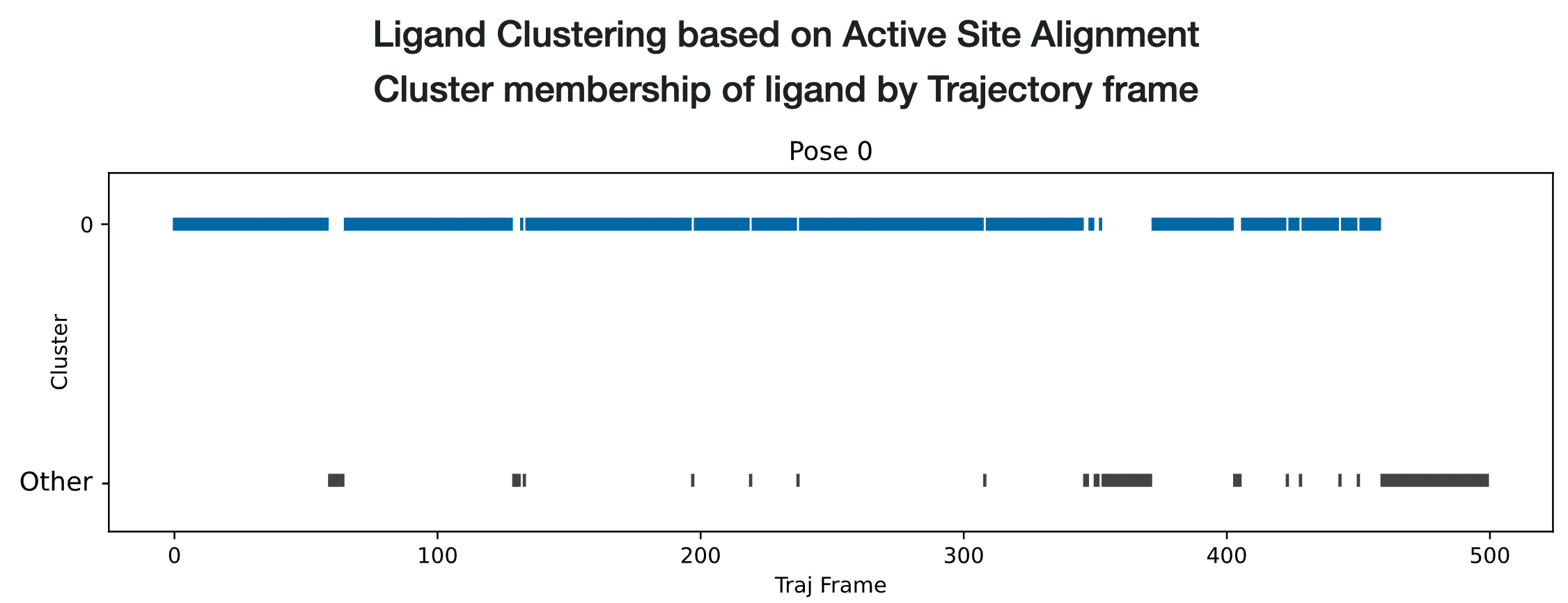
Strip Chart results for ligand 35 (single pose)
The strip chart shows a time course over the MD trajectory, always maintaining the same color scheme as in the interactive graphic: blue for cluster 0. Additionally, cluster outliers, which are ligand configurations that do not belong to any cluster, are shown in black. The chart simply shows the cluster occupancy of each frame, telling us that the trajectory spent most of the time in the blue Cluster 0, occasionally sampling outliers. It seems like quite a stable pose!
The two tables below the strip chart, shown in Cluster/Pose information for ligand 35 (single pose) describe a relationship between each cluster found in the MD for the ligand and the starting poses.
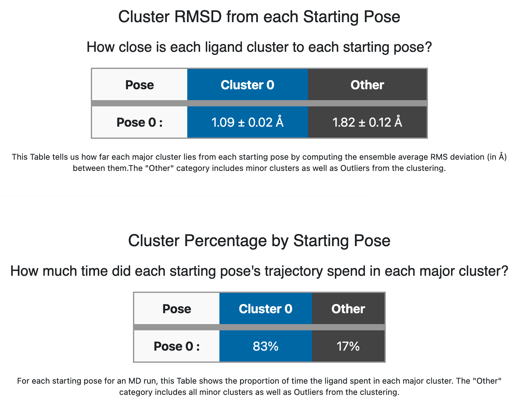
Cluster/Pose information for ligand 35 (single pose)
With only one pose used for this run, the tables are terse, but below when we look at 6 input poses for the same ligand, they will be more informative. The upper table “Cluster RMSD from each Starting Pose” describes how closely each cluster stays to the starting pose: the blue Cluster 0 sticks closely to the initial pose (1.09 Å RMSD). The second table “Cluster Percentage by Starting Pose” simply describes the occupancy that we see in the strip chart: the ligand spends 83% of its time in cluster 0. These figures tell us the blue Cluster 0 is stable and stays close to the initial pose.
MCL1 ligand 35: 6 input poses
Now we will look at the results of another run on the same ligand 35, but this time with 6 different input poses: 3 related poses with the methyl “up” in the upper panel of Figure Input poses for the 6-pose run and 3 related poses with the methyl “down” in lower panel of the same Figure. The “up” and “down” poses are only differentiated in the Figure for clarity; in the input file all 6 poses are together as the 6 conformers of the ligand 35 molecule. Poses 0, 3, and 5 have the methyl “down” and poses 1, 2, and 4 have the methyl “up” (this will be important later). The question we might be asking here is whether the “up” methyl or “down” methyl is preferred, and which of the input poses (if any) is preferred. Of course, we want to see if the preferred cluster by MD still retains the binding interactions we thought were good enough to carry ligand 35 along up to this point.
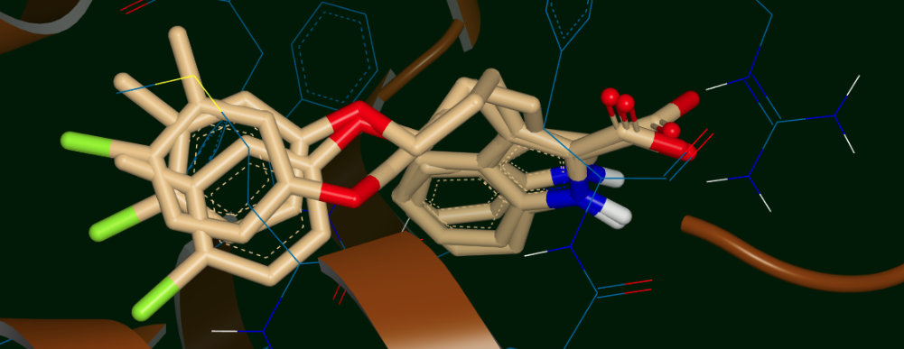
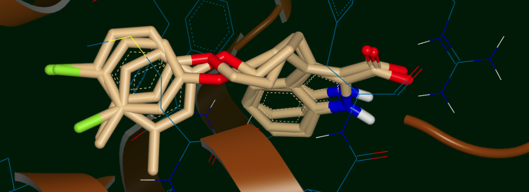
Input poses for the 6-pose run: 3 with the methyl “up” (top) and 3 with the methyl “down” (bottom)
Once the run is completed, again we go to the job results page, not shown here because it is so similar to what we saw with the single-pose example in Figure Input poses for the 6-pose run (above). Selecting the third tab (”FLOE REPORT”), there is still only a single tile for the single ligand; the results for all 6 poses have been aggregated and analyzed together for that ligand. The atom colors corresponding to the calculated B-factors will often be a lot “hotter” (more red) for multiple-pose inputs because trajectories for diverse poses are aggregated together, often giving higher per-atom fluctuations. Click on the tile to drill down into the detailed analysis, resulting in Figure Detailed results for ligand 35 (6 poses):
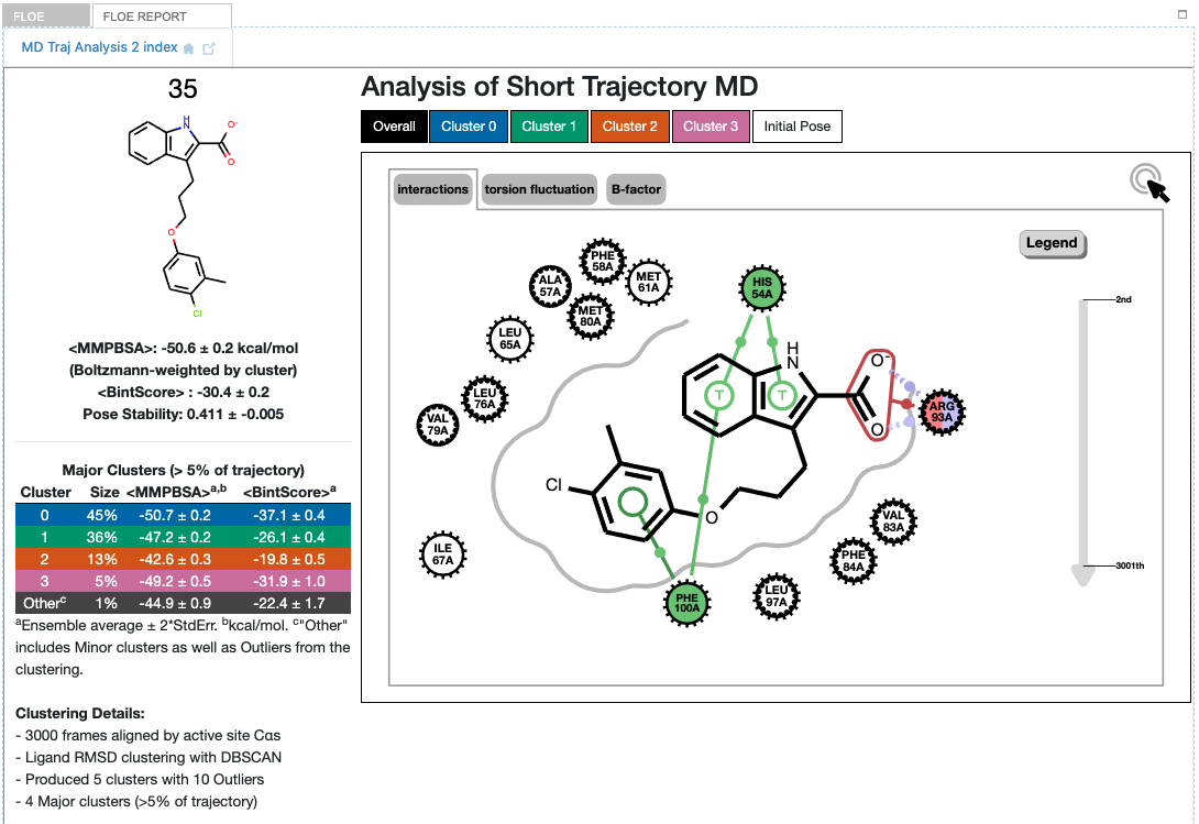
Detailed results for ligand 35 (6 poses)
The results look quite different from the single-pose case although the binding interactions are mostly the same (the 2D representation shows a different orientation). There are now four major clusters resulting from the combined trajectories. As a reminder, the results are not deterministic: In you run this same MD again, in principle you could get slightly different results. Nevertheless, the results are interpreted in the context of the sampling obtained.
The table to the left of the graphic gives key information on each cluster. The blue cluster 0 is dominant, accounting for 45% of the trajectory and with the best (lowest) ensemble MMPBSA and Bintscore. Cluster 1 (green) is second largest at 36%, and has less good MMPBSA score and BintScore. Cluster 2 (orange) at only 13% abundance scores the worst compared to the others, while Cluster 3 (pink) scores second best by both MMPBSA and BintScore even though it is the smallest cluster at 5%. How do these clusters relate to the different input poses?
Scrolling down to the strip chart, shown below in Figure Strip Chart results for ligand 35 (6 poses), we see the time course over the MD trajectories for all starting poses concatenated and analyzed together. The strip chart and the table below it (table Cluster Percentage by Pose for ligand 35 (6 poses) both point to a clear grouping by pose: poses 0, 3, and 5 show predominantly cluster 0 occupancy (blue), and poses 1, 2, and 4 show predominantly cluster 1 occupancy (green).
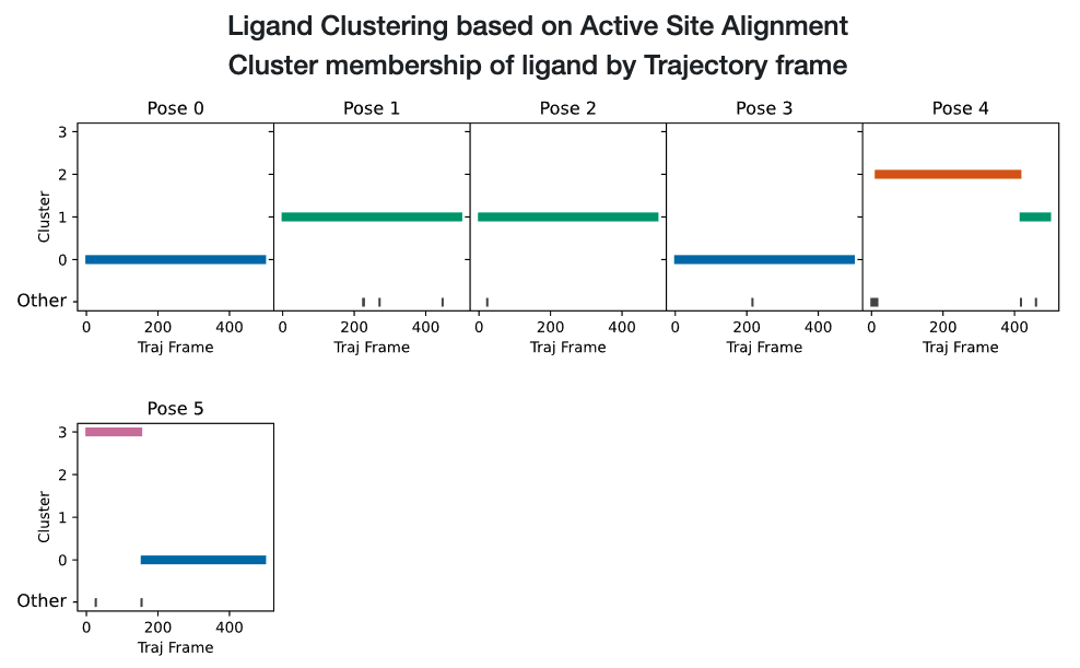
Strip Chart results for ligand 35 (6 poses)
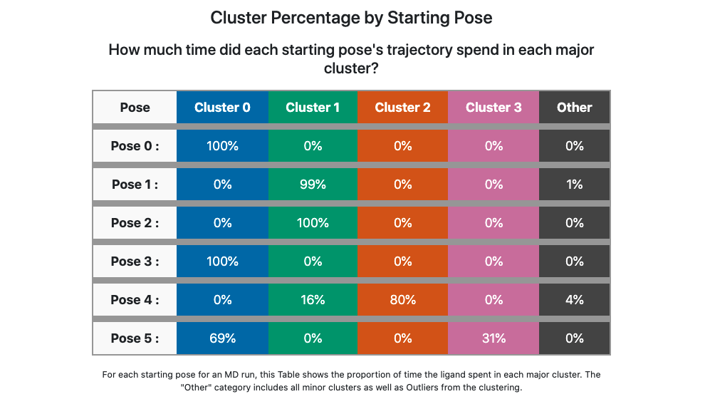
Cluster Percentage by Pose for ligand 35 (6 poses)
The former poses correspond to the methyl “down” starting poses and the latter to the methyl “up” starting poses, which we can confirm in the Orion 3D page. While the short trajectories in this run (2 ns for each pose) do not allow interconversion between methyl “up” and “down” poses, it appears that the 3 poses in each category have collapsed to a single dominant cluster. How close is the cluster to any of the starting poses? This answered by the Table Cluster RMSD from Pose for ligand 35 (6 poses).
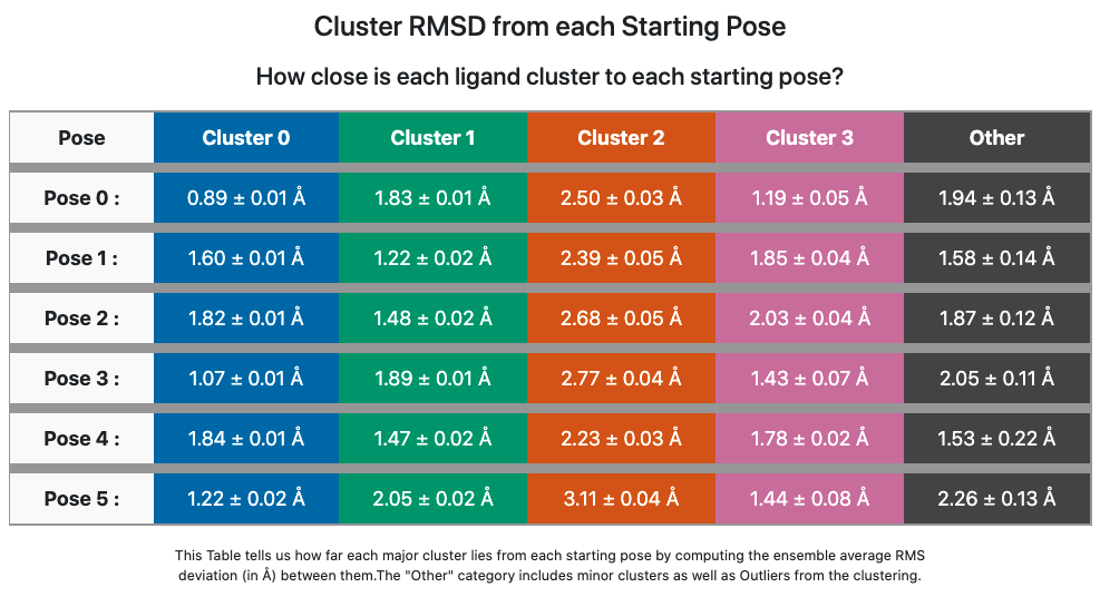
Cluster RMSD from Pose for ligand 35 (6 poses)
This table confirms that cluster 0 is quite close to the starting poses (0, 3, and 5) that contributed to it, though slightly closer to Pose 0. Cluster 1 is still within 2 Å of 5/6 poses, but closest to Pose 1 out of all.
We can visually confirm this by selecting the output dataset (in the “Data” tab of Orion) and then going to the “3D” tab. Under the list of structures for ligand 35, the starting poses are conformers under the molecule named simply “35”. Unfortunately the conformer number in this structure are off by 1, starting from “1”, compared to the analysis, which starts from 0! This bug will be fixed in a future release. The average and median for each cluster appear as a separate protein-ligand complex, labeled accordingly (for example “35_clus0_Avg” for the average of cluster 0). Selecting starting poses corresponding to “down” poses 0, 3, and 5 (i.e. conformers 1, 4, and 6) and displaying them with the average for cluster 0 (“35_clus0_Avg”) gives the upper panel in Figure Starting Poses and Cluster Averages for ligand 35. Selecting starting poses corresponding to “up” poses 1, 2, and 4 (i.e. conformers 2, 3, and 5) and displaying them with the average for cluster 1 (“35_clus1_Avg”) gives the lower panel. Interestingly, with the averages color by calculated B-factor it is obvious that the “down” cluster is markedly more stable in the active site than the “up” cluster, as well as being more energetically favorable by MMPBSA and BintScore.
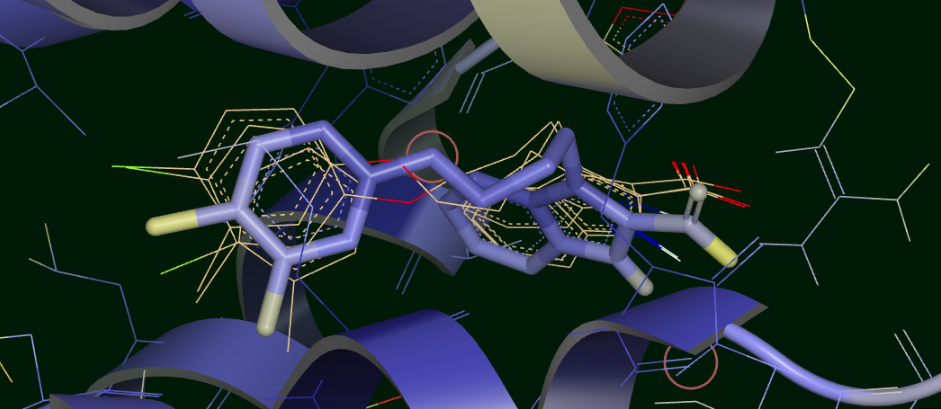
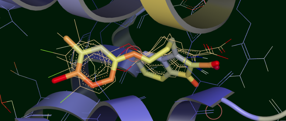
Starting Poses and Cluster Averages for ligand 35
These visually confirm what we had seen emerging from the analysis: the 6 poses collapse into a predominant methyl “up” and methyl “down” pose. Cluster 0 lies close to one of the starting poses, but Cluster 1 lies in between two of the starting poses. Cluster 0 has a more stable pose than Cluster 1, and the ensemble MMPBSA energies and BintScores also favor Cluster 0.
Understanding the results for a set of ligands
Finally we will look at how to visualize the results for a 11-ligand subset that spans the range of activities for the MCL1 dataset. Each of 11 ligands has 5 reasonable input poses from docking. The whole subset will be run in the same job in the “Short Trajectory MD with Analysis” floe. which will consist of 11 ligands * 6 poses each = 66 MD run of 2ns each. Selecting the output dataset in the “Data” tab and moving to the “Analyze” tab, the results for the entire dataset can be viewed at once as in Figure Analyze page for MCL1 dataset:
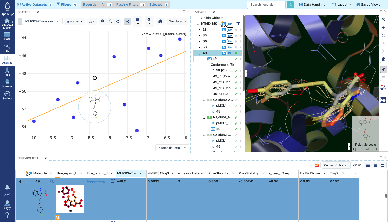
Analyze page for MCL1 dataset
There are a lot of results showing in this page, encompassing both numerical and 3D information. The 3D info is brought in by selecting Analyze with 3D under the Layout pull-down menu at the top right. The axes of the scatterplot were selected to display the experimental deltaG (included as SD tag ‘r_user_dG.exp’ on the input ligands) on the x axis and the Boltzmann-weighted ensemble MMPBSA value on the y axis. In the 3D visualizer, select ligand 49 and unroll the list of associated structures. The point in the scatter plot corresponding to ligand 49 and the corresponding line in the spreadsheet is highlighted. In the 3D window, the 5 initial input poses for ligand 49 are under Molecule “49” and display in in gold if selected. Turn on the protein-ligand average structures for Clusters 0 and 1, which will be colored by B-factor as before. This way we can compare the poses to the representative average for each cluster, helping us to evaluate and prioritize that ligand. To call up the detailed MD analysis once again, go to the spreadsheet row for ligand 49, and under the column titled Floe_report_URL click on the little square to open up another tab in your browser with the same detailed analysis Floe report as we saw above.
There is a lot of information to look at in the results from the Short Trajectory MD with Analysis Floe, but this should get you started. We emphasize that a lot of the analyses can only be interpreted qualitatively at this stage, but nevertheless we feel that the sampling of both protein and ligand configurations at physiological temperatures in the context of explicit water solvation can help validate the initial input pose(s).
Footnotes