FE-NES Tutorial

FE-NES for binding affinity prediction can be executed using the FE-NES for Binding Affinity Prediction Floe. It implements the nonequilibrium switching (NES) method to compute relative binding free energies (RBFE) of ligands to a given target. The NES method is based on the Jarzynski equality ([Jarzynski-1997a]; [Jarzynski-1997b]) and is a nonequilibrium approach to compute free energy differences. For more details on the theory behind the NES method, please refer to the FE-NES theory section.

FE-NES for Binding Affinity Prediction Floe

The FE-NES for Binding Affinity Prediction Floe implements the NES method to compute RBFEs of ligands to a given target. From these RBFEs, the floe computes \(\Delta G\)s of the ligands. It does not require a map of edges to be provided, as it can construct a map using the provided ligands. The floe is designed to be user-friendly and requires minimal input from the user. All other parameters that can be modified by the user have sensible default values.

You must provide a minimal dataset of posed ligands and a target protein.

You can provide an additional combination of these inputs to skip specific operations in the floe:

• A Custom edge map, for which the Edge Mapper for RBFE calculations Floe can be used. This dataset contains the edge information for the RBFE calculations to be carried out. There is also an option to provide custom edges via a text file. If provided, the floe will skip the edge map construction step and use the provided edges for the RBFE calculations.

• An Existing End-state Simulation dataset, which contains the bound and unbound equilibrium simulation data for the ligands. If provided, the floe will skip the equilibrium simulations and proceed directly to the NES calculations.

You can also provide experimental binding affinity values for the ligands. These are used to offset the \(\Delta G\)s to the mean of the experimental binding affinity values, thereby providing you with predicted affinity values that can be conveniently compared with the experimental numbers. The floe can read these values from a dataset or a text file; if using a dataset, you must specify the column containing the affinity values and their units. See Experimental Affinity Inputs for more details on how to provide experimental affinity values in either format.

How to Use the Floe

Input files for this tutorial

You can use these files to follow this tutorial:

• Target protein (Tyk2)

• 6 Ligands in their bound poses

• Pre-made edge map of Tyk2 ligands

• Experimental affinities of Tyk2 ligands

Lauching the FE-NES for Binding Affinity Prediction Floe

Instructions to locate and launch the FE-NES for Binding Affinity Prediction Floe in Orion can be found here.

Minimal Inputs for a New FE-NES Calculation

The minimal inputs required to run an FE-NES calculation are entered in the Main Settings section of the Job Form. You can either start a new calculation from a target protein and posed ligands or reuse equilibrium simulations generated in a previous FE-NES run.

To perform a new FE-NES calculation, provide the following inputs:

Target Protein

A dataset containing the protein prepared up to MD standards, which includes chain capping, all atoms in protein residues (including hydrogens), and missing protein loops resolved or capped. Protein side chain formal charges and protonation determine the tautomeric states. Additionally, it is important to include cofactors and structured internal waters. We strongly recommend using the SPRUCE Protein Preparation Floe.

Posed Ligands

A dataset containing ligands with 3D coordinates, all atoms, and correct chemistry. In particular, bond orders and formal charges should be correctly assigned.

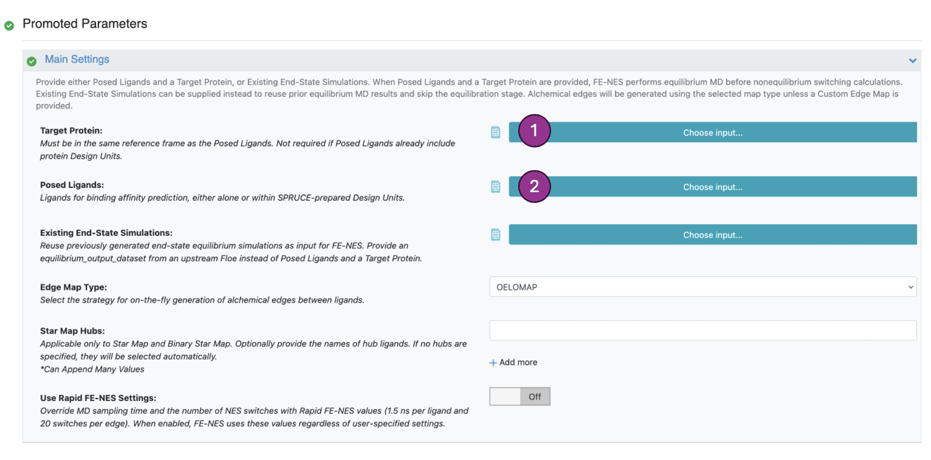
Figure 1. Minimal inputs for the FE-NES for Binding Affinity Prediction Floe.

Target protein input

Two things must be noted about the target protein input:

1. The target protein dataset should contain only ONE record. Output from the SPRUCE - Protein Preparation Floe can produce a dataset with multiple records, with each record corresponding to a different pocket size of the protein. In that case, you must select the record corresponding to the pocket size of interest and provide it as input to the floe.

2. The target protein input is actually optional, but if it is not provided, the protein must be present in the datasets provided as input to Posed Ligands. These datasets must contain a OEDesignUnit in each record; each design unit corresponds to a bound complex of every ligand with the target protein. If a protein cannot be found, an error is raised and the floe fails. If the protein is provided as input, and the protein is also present on the ligand input datasets, the protein input will supersede.

The POSIT - Ligand Guided Small Molecule Posing Floe is able to produce ligand datasets with a target protein included.

Successful job submission

After you have loaded these files, click the “Start Job” button on the Job Form to begin the floe. It takes approximately 2 hours, 30 mins for the job to complete with the inputs provided in this tutorial (without the Rapid FE-NES mode).

Outputs from FE-NES

Details about the output from the FE-NES for Binding Affinity Prediction Floe are accessible from the following:

• Four primary Floe Reports

• Three datasets

• One tar.gz file

When the job completes, these outputs become available under Results in the job information on the Jobs tab of the Floe page.

The main Floe Reports are:

Relative Affinity Predictions Report

This report includes all the edges with successful RBFE calculations in thumbnails. When you click on an edge, you can see the edge’s work distributions, free energy changes, and overlap estimates.

Edge Map Diagram with Predictions

This report shows the predicted and experimental \(\Delta \Delta G\)s for each edge, as well as the predicted and experimental \(\Delta G\)s for each ligand. These values are illustrated on a graph. The edges are colored based on the work overlap estimates.

Affinity Predictions Report

This report lists the predicted \(\Delta G\)s and \(\Delta \Delta G\)s. If experimental values were provided in the input, the report also shows the experimental values and compares them with the predicted values. The report also provides statistical metrics for the comparison.

Trajectory Downloader

This report provides a link to download the trajectory files for the bound and unbound equilibrium simulations. The files (in .tar.gz format) can be downloaded for offline analysis. See Downloading Trajectories from Floe Reports for details.

The three primary datasets (with default names) are:

affinity_predictions

This dataset contains the predicted \(\Delta G\)s of each ligand (in column Pred dG) and the associated uncertainty (in column Pred dG Err).

relative_affinity_predictions

This dataset contains the predicted \(\Delta \Delta G\)s of each edge (in column Pred ddG) and the associated uncertainty (in column Pred ddG Err). It also contains the work overlap estimates for each edge.

md_output

These datasets contain the bound and unbound equilibrium simulation data for each ligand. Each record in the dataset has a unified structure with information for both bound and unbound simulations of a ligand.

Additional datasets

Other datasets may be produced if there is a failure or if specific parameters are requested.

1. md_recovery

2. Failed Output for FE-NES for Binding Affinity Prediction

3. edge_map

4. all_possible_edges

The one file output (with default name) is:

fe_nes_results_archive.tar.gz

This tar.gz file contains several .csv and .txt files, which contain information available in the Floe Reports. These ASCII files can be used for further analysis of the results. The file also contains the Floe Reports in .html format.

Additional output files

Additional output files are:

1. fe_nes_recovery_binary: Can be used as input in the Result Recovery for FE-NES Floe

2. edge_map.txt

For the inputs used for this tutorial, the results produced are shown in Figures 2–9. The Floe Reports can be found by clicking on the job name in the Jobs tab of the Floe page to access the Reports section of the detailed job information (Figure 2).

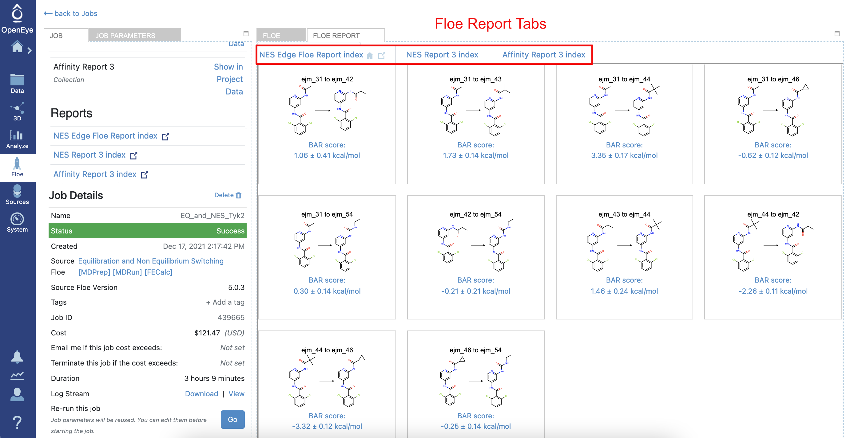
Figure 2. The job outputs and Floe Report for the FE-NES for Binding Affinity Prediction Floe.

There are two main sections in the Affinity Predictions Report. In its top section (Figure 3), experimental and predicted affinities are compared. Here, a graph of \(\Delta G_{Experimental}\) versus \(\Delta G_{Predicted}\) is shown. This graph is only plotted if experimental affinities were provided and the ligand edge map is connected enough to make affinity predictions. Additionally, the graph data are tabulated and different statistical metrics, such as correlation metrics and linear models, are shown.

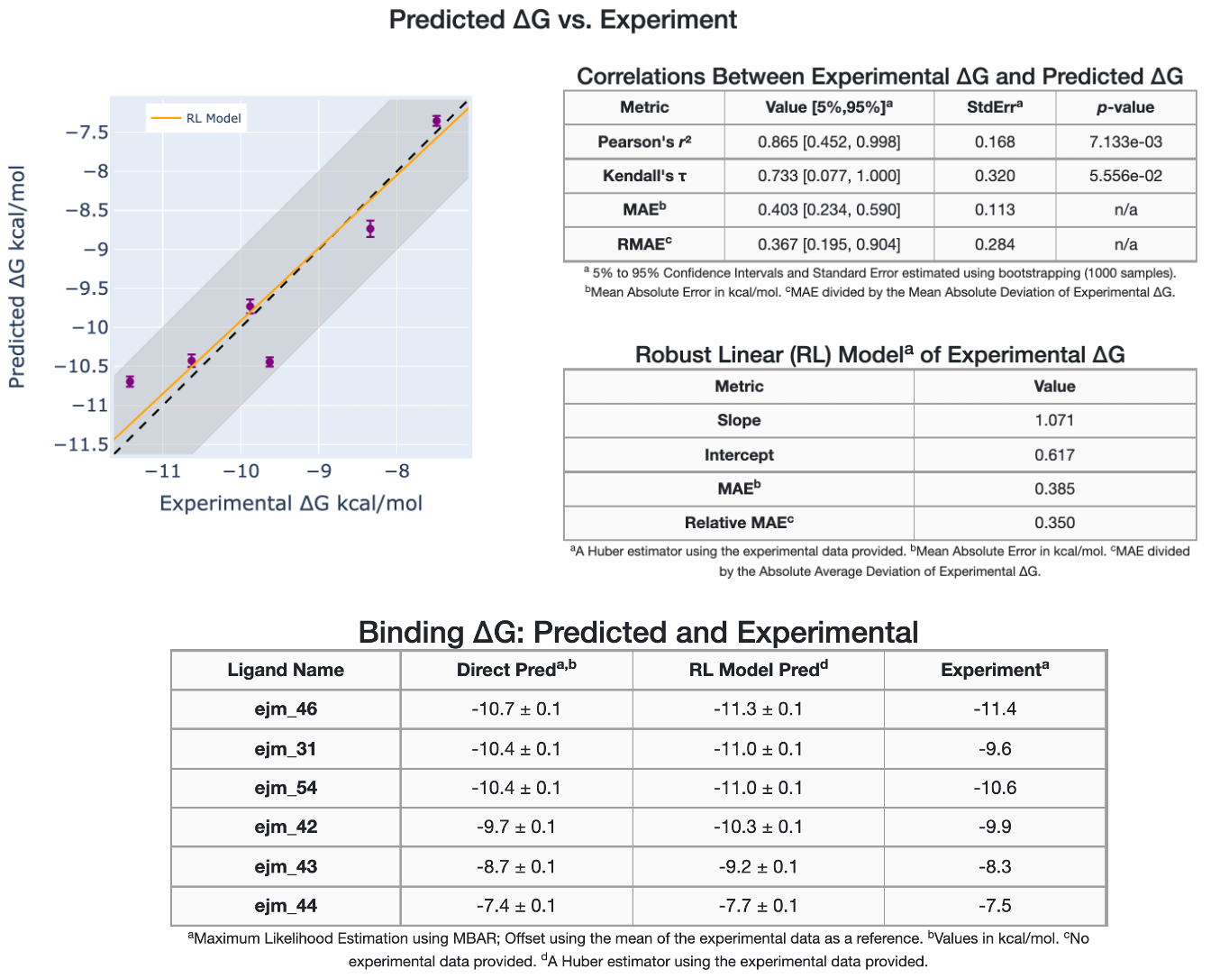
Figure 3. Experimental versus predicted affinities.

The bottom section of the Affinity Predictions Report shows a comparison between the experimental and predicted relative binding affinities, \(\Delta\Delta G_{Experimental}\) versus \(\Delta\Delta G_{Predicted}\), in addition to statistical metrics (Figure 4).

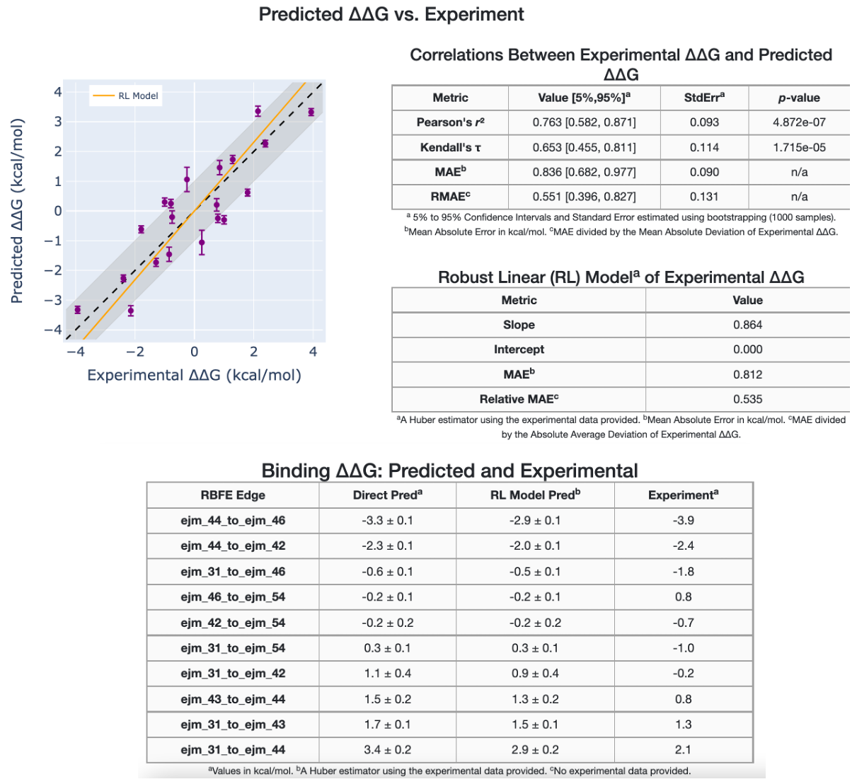
Figure 4. Experimental versus predicted relative binding affinities shown in the Affinity Predictions Report.

To investigate the RBFE values, you need to locate the Relative Affinity Predictions Report. Here, the thumbnails corresponding to each edge can be seen. On the search bar, type the name of any ligand to find the edges containing that ligand. In Figure 5, ejm_46 is typed to see all edges containing the ligand ejm_46.

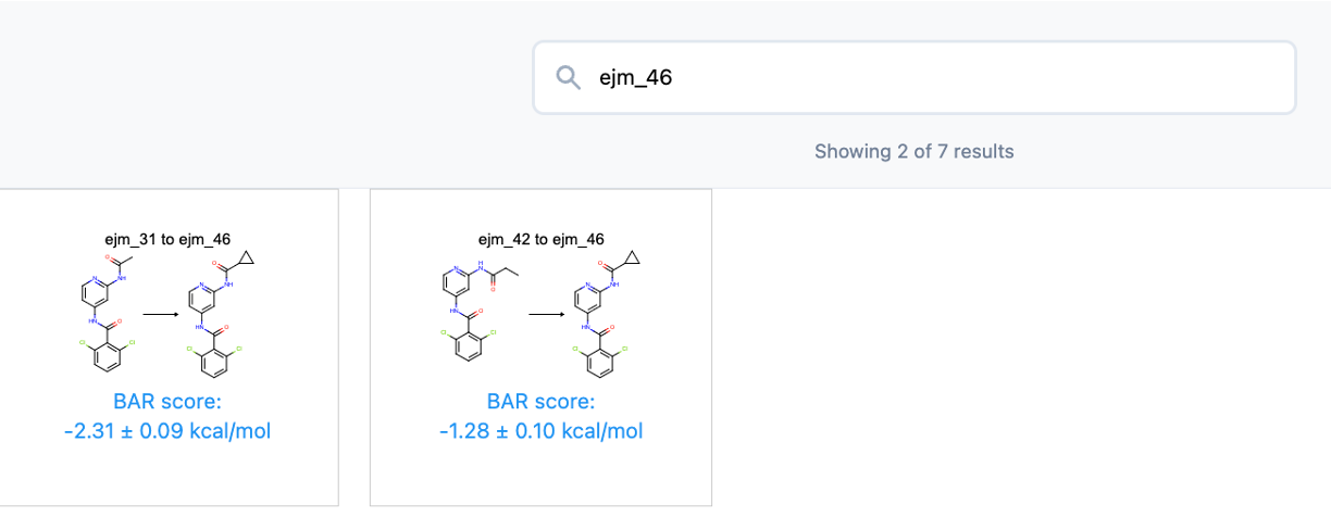
Figure 5. Searching for edges containing the ligand ejm_46 in the Relative Affinity Predictions Report.

After clicking a thumbnail (e.g., ejm_42 to ejm_46), you are led to another page where details about the alchemical switches between the two ligands can be found. This page (e.g., Figure 6) includes work distributions in the bound and unbound stages (computed using the Bennett Acceptance Ratio (BAR) method), the free energy in these stages, and the \(\Delta\Delta G\) of that edge.

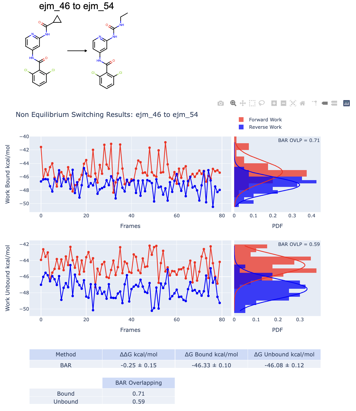
Figure 6. An example of data from a good RBFE calculation for the ligand ejm_42 to ejm_46.

This Floe Report page shows the FE-NES results for a single edge, that is, one ligand pair. The upper and lower panels refer to the bound and unbound legs of the transformation, respectively. For each leg, the blue and red graphs plot the forward and reverse switching work values obtained from the selected equilibrium starting frames, and the corresponding probability distributions are obtained by binning those work values. The overlap between the two work distributions is estimated with the BAR and reported in the plot and in the accompanying table. From these work values, the free energy changes \(\Delta G_{Bound}\) and \(\Delta G_{Unbound}\) shown in Figure 6 are estimated, and the relative binding free energy for this edge is obtained as \(\Delta\Delta G = \Delta G_{Bound} - \Delta G_{UnBound}\), which is also reported in a table.

The Edge Map Diagram with Predictions shows all the compounds involved in the FE-NES calculation. It offers a complete visualization of the edge map (Figure 7). The edges are colored based on the work overlap estimates.

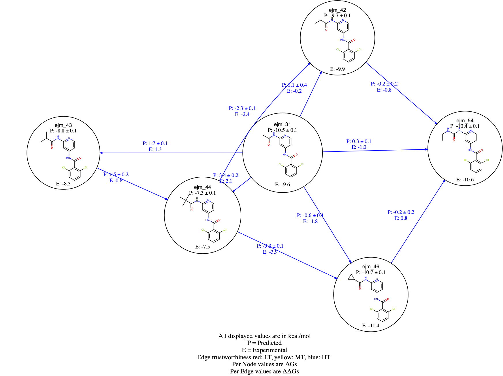
Figure 7. The Edge Map Diagram with Predictions showing the edge map for all compounds involved in the edges.

Each edge reports the predicted (P) and, where available, the experimental (E) \(\Delta \Delta G\)s, while each compound reports the predicted (P) and, where available, the experimental (E) \(\Delta G\)s. Edges are colored by their BAR work overlap estimate: blue if both the bound and unbound overlaps exceed 0.2, yellow if only one of them does, and red if neither does. Clicking on an edge opens the page shown in Figure 6.

tar.gz file output

The tar.gz contains all the \(\Delta \Delta G\) and \(\Delta G\) data in .csv file formats that can be used for a more detailed analysis. It also contains all the floe reports in .html reports, except the Trajectory Downloader report.

File from this tutorial

The result files generated for the Tyk2 receptor can be downloaded from this tar.gz file: Tyk2_floe_results.tar.gz.

The Trajectory Downloader report (Figure 8) provides a link to download the trajectory files for the bound and unbound equilibrium simulations. It can also be opened from the Reports section of the detailed job information, which can be found by clicking on the job name under the Jobs tab. The trajectories of bound and unbound simulations for each ligand can be downloaded separately by clicking on a download link. For instructions on downloading, uncompressing, and converting trajectories for offline analysis, see Downloading Trajectories from Floe Reports.

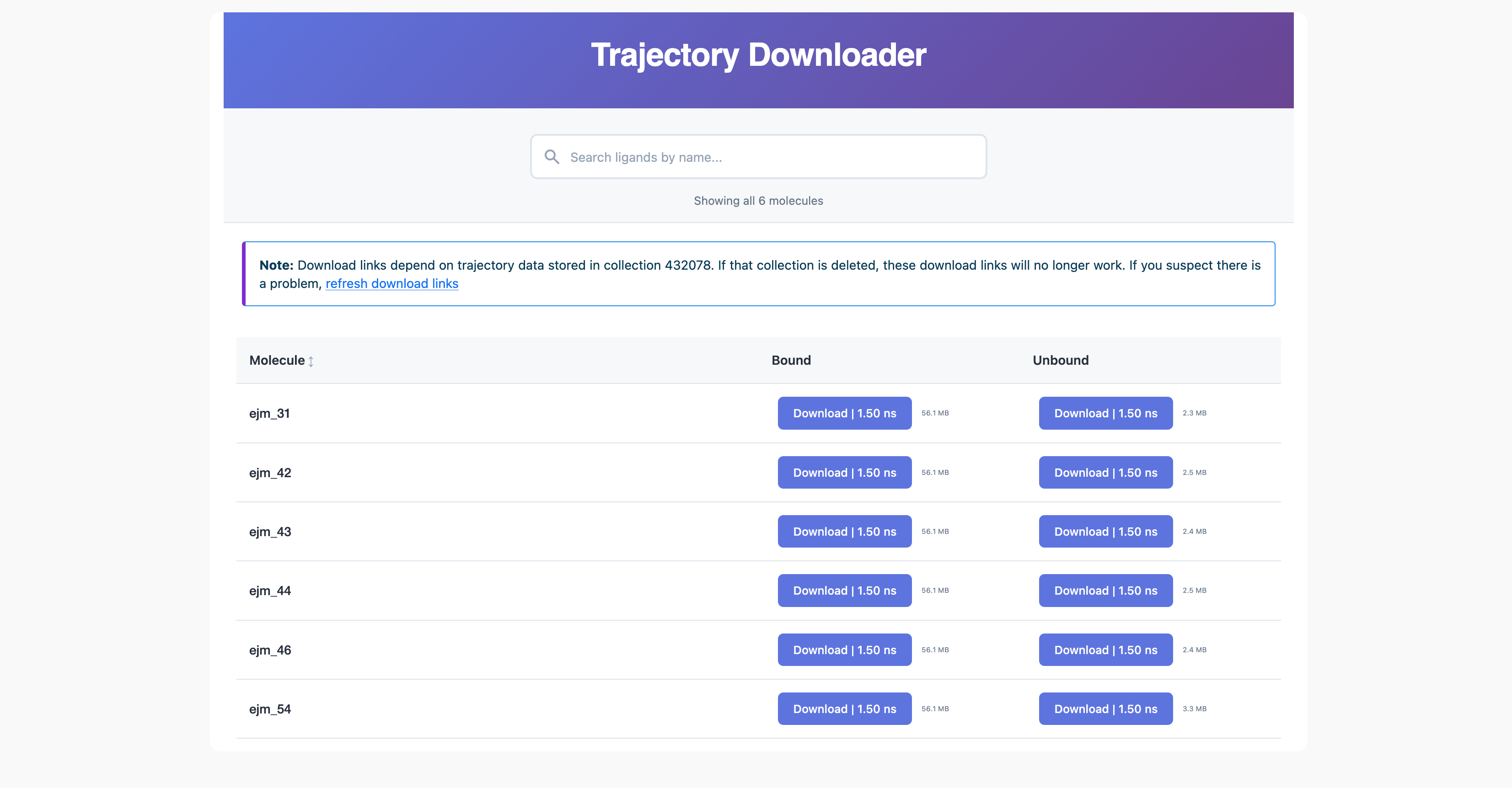
Figure 8. The Trajectory Downloader report.

Additional Inputs for FE-NES

The defaults for the parameters in the sections following the Main Settings can be changed to customize the FE-NES calculations.

Edge Map Type

You select an Edge Map type to specify the method used to construct the edge map for the RBFE calculations.

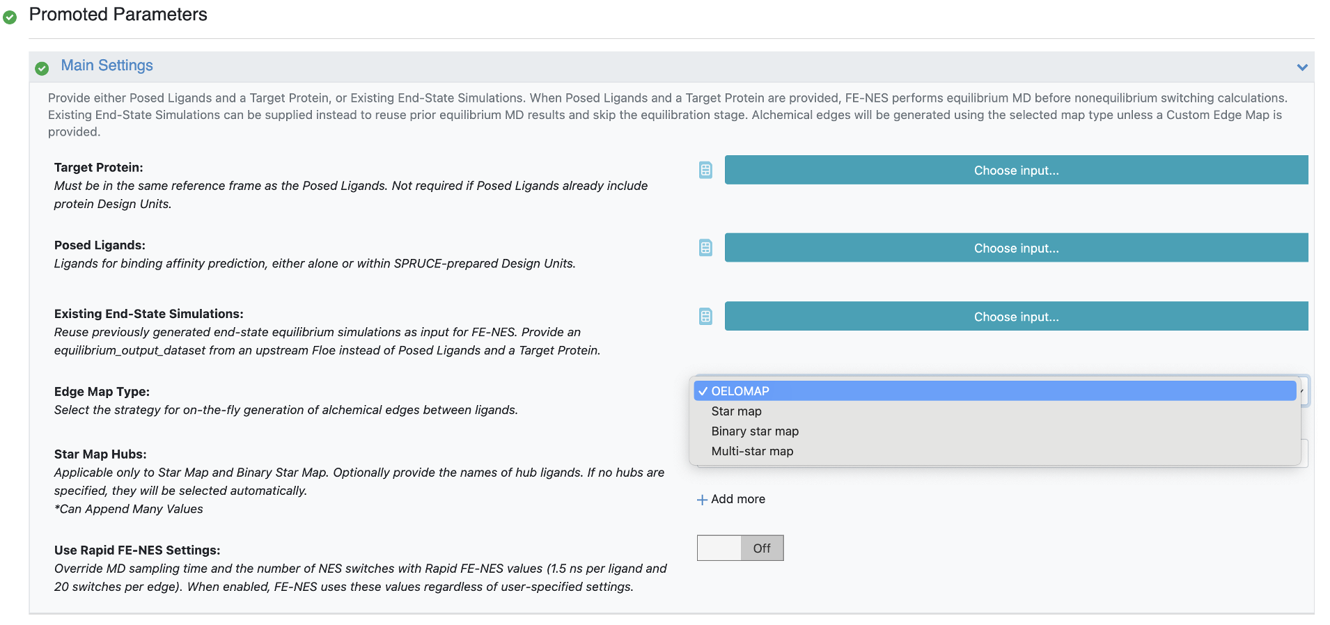
Figure 9. Edge map type choices for the FE-NES for Binding Affinity Prediction Floe.

It can be selected from the following options (Figure 9):

1. OELOMAP (default): This option constructs an edge map using the OpenEye OELMAP algorithm, which connects ligands based on their chemical similarity.

2. Star Map: This option constructs an edge map using a star topology, where one ligand is chosen as the hub and all other ligands are connected to it.

3. Binary Star Map: This option constructs an edge map using a binary star topology, where two ligands are chosen as hubs and all other ligands are connected to one of the hubs.

4. Multi Star Map: This option constructs an edge map using a multi-star topology, where multiple ligands are chosen as hubs and all other ligands are connected to one of the hubs.

Hub Selection for Star Map Edge Types

To specify the hub ligands to be used for the edge map construction, select Star Map or Binary Star Map edge map types. The hub ligand(s) must be present in the set of provided posed ligands. If no hub ligands are specified, the floe automatically selects hub ligands based on internal heuristics.

For the Star Map, only one hub ligand must be specified (if you choose to avoid automatic hub selection). The name of the hub ligand should be entered as an input to the Star Map Hubs parameter.

For the Binary Star Map, two hub ligands must be specified (if you choose to avoid automatic hub selection). The names of the two hub ligands should be entered as inputs to the Star Map Hubs parameter. The second hub ligand can be specified in the second text field that appears when you click on the “Add More” button.

For the Multi Star Map, hub ligands should not be specified. The floe automatically selects hub ligands based on internal heuristics.

Error on hub selection

If you specify hub ligands that are not present in the set of provided posed ligands, the floe will raise an error and fail. The floe also fails when the Edge Map type is set to OELOMAP or Multi Star Map and hub ligands are specified, as these edge map types do not require user-specified hubs.

Running Rapid FE-NES

In the Main Settings section, the FE-NES Floe can be asked to run in Rapid FE-NES mode by turning on the Use Rapid FE-NES Settings switch.

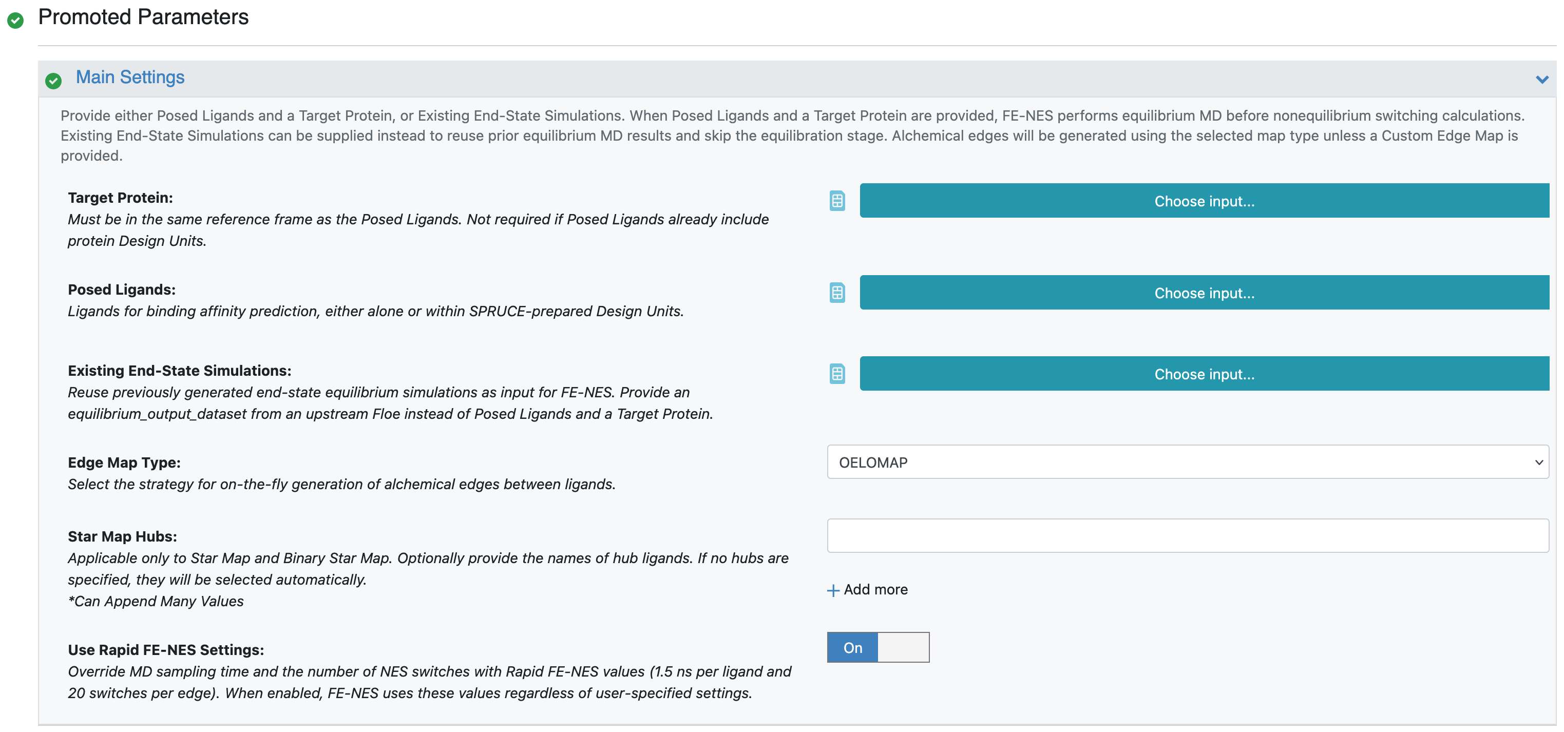
Figure 10. Rapid FE-NES settings for the FE-NES for Binding Affinity Prediction Floe.

When this switch is turned on, the floe will use a set of predefined parameters that are optimized for speed and cost. These parameters include:

1. Reduced MD sampling time (1.5 ns instead of 6 ns)

2. Reduced number of alchemical switches (20 instead of 80)

To see more details, see the Rapid FE-NES tutorial.

To control the parameters used in the Rapid FE-NES mode separately from the switch, see the parameters in the End-State Simulation Settings and Alchemical Switching Settings sections.

Reusing Existing End-State Simulations

Instead of providing a target protein and posed ligands, you can also provide an input dataset containing existing end-state simulations, which contains previously generated bound-state and unbound-state equilibrium MD simulations.

When this input is provided, the floe reuses the existing equilibrium simulations and skips the equilibration stage, proceeding directly to the nonequilibrium switching calculations.

It also constructs an edge map using the ligands present in the existing end-state simulations dataset if a custom edge map is not provided.

Usefulness of Existing End-State Simulations

Reusing existing end-state simulations can save time and cost.

1. This enables use of data generated earlier for the same target.

2. It also allows reevaluation by FE-NES on extended equilibrium simulations, which can improve the accuracy of the RBFE predictions. See the Extend MD Simulations tutorial for more details on how to extend equilibrium simulations.

Note

When the existing end-state simulations dataset is provided, the Target Protein and Posed Ligands inputs are not required. However, if these inputs are provided, the floe will ignore them and use the existing end-state simulations.

Custom Edge Map

A custom edge map can be provided via a dataset or a text file. If provided, the floe will skip the edge map construction step and use the provided edges for the RBFE calculations.

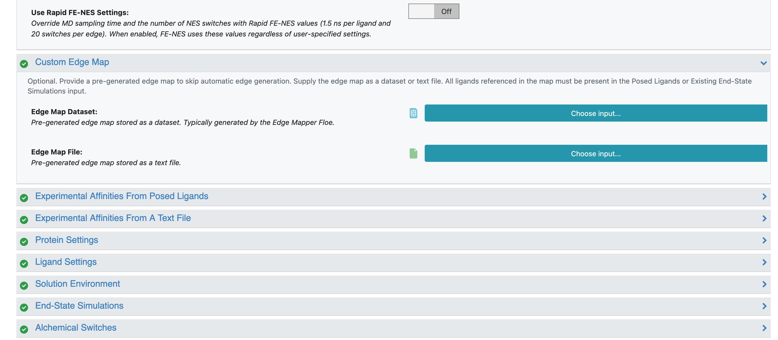
Figure 11. Custom edge map input for the FE-NES for Binding Affinity Prediction Floe.

It is advised that a dataset containing edges be generated using the Edge Mapper for RBFE calculations Floe. It is guaranteed to produce a dataset with the requisite fields.

If a text file is provided, it must be in the following format:

[ligand1] >> [ligand2]
[ligand3] >> [ligand4]
# Commented lines are ignored [ligand5] >> [ligand6]
...

where each line contains a pair of ligands that form an edge. The ligands must be present in the set of provided posed ligands.

File over dataset precedence

If both a dataset and a text file are provided for the custom edge map, the floe will use the file rather than the dataset.

Providing Experimental Affinities for Ligands

Experimental affinities of ligands can be read directly from the Posed Ligands dataset. However, you must specify the column of the dataset, which contains affinity data and, optionally, the error in the affinity data. The units of the affinity data must also be specified.

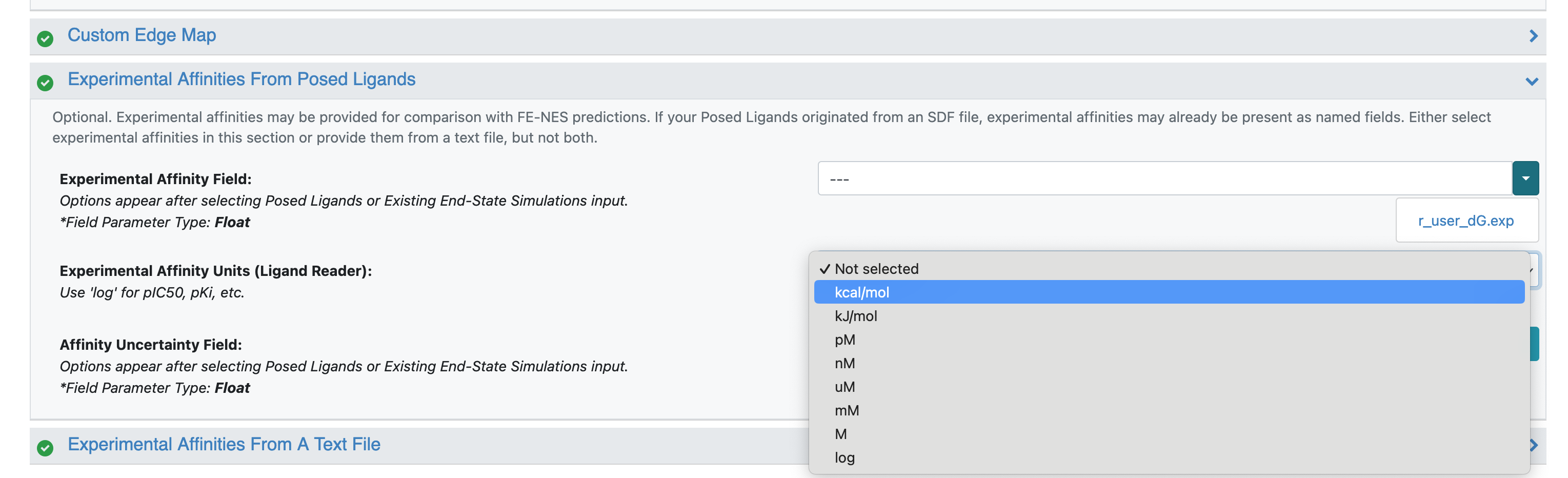
Figure 12. Experimental affinities input using column selection for the FE-NES for Binding Affinity Prediction Floe.

An example is shown in Figure 12. You can select a column that has the experimental affinities for the Experimental Affinity Field (r_user_dG.exp in the example) and the correct unit from the drop-down menu for Experimental Affinity Units. If the dataset contains a column with error values, it can be selected for the Affinity Uncertainty Field. If unavailable, the error is assumed to be zero.

Regardless of the units of experimental affinities, the predictions from the FE-NES Floe are always reported in the units of kcal/mol. In the Affinity Predictions Report, the original experimental affinities are listed alongside their values in kcal/mol in addition to the predicted affinities in kcal/mol. This allows for easy comparison between experimental and predicted values. The conversion formulas are provided in the Affinity Conversion Table section.

Load dataset first to see columns

The columns of the dataset will only be visible after the dataset is loaded. If the dataset is not loaded, the drop-down menu for column selection will be empty.

If the experimental affinities are not present in the Posed Ligands dataset, they can be provided via a text file. The parameters are available under the Experimental Affinities From a Text File group.

More details for providing experimental affinities to the FE-NES for Binding Affinity Prediction Floe can be found in Experimental Affinity Inputs.

Protein Settings and Ligand Settings

Settings for the protein and ligand force fields, and several other parameters related to their MD simulations, can be modified in the Protein Settings and Ligand Settings sections.

In the Protein Settings section, you can choose the protein force field to be used for the simulations. The default is Amber14SB, but other options are available in a drop-down menu.

You can also request tumbling restraints to be applied on the bound complex during the equilibrium MD simulations. This is done by turning on the Restrain Protein Motion switch, in the Protein Settings section.

Restraining motion in rectangular solvation box

When a rectangular solvation box is used, we recommend restraining protein motion. A guardrail is set up within the floe to ensure that these restraints are applied when a rectangular solvation box is used. You can remove the guardrail by turning the Checker Bypass on. This parameter is not promoted; it can be found in the Cube parameters of the Bound Protein Ligand MD Health Checker.

In the Ligand Settings section, you can choose the ligand force field to be used for the simulations. The default is OpenFF 2.2.1, but other options are available in a drop-down menu. You can also provide a custom ligand force field file in SMIRNOFF XML format.

The floe runs the ligands through a partial-charge reassignment protocol using the AM1BCC-Elf10 method by default. If you want to use the ligand partial charges provided in the input dataset, they can be turned off with the Reassign Ligand Partial Charges switch.

Solution Environment Settings

Parameters related to the solution environment for the MD simulations can be modified in the Solution Environment parameters.

1. Unit Cell Geometry - (cubic) The only other option is rectangular. The choice of unit cell geometry only affects the solvation box used for the MD simulations of the ligands found. For unbound ligands, cubic boxes are always used.

2. Unit Cell Padding - (6 Å) This controls the distance between the solute and the edges of the solvation box.

3. Solution Density - (1.03 g/mL) This controls the density of the solvent in the box.

4. Salt Concentration - (150 mM) This controls the concentration of NaCl salt in the solution. The floe automatically adds these counterions to neutralize the system.

Solvent model

The solvent model is TIP3P.

End-State Simulation Settings

Settings related to the duration of the equilibrium MD simulations, sampling interval, timestep, and so on can be modified in the End-State Simulations parameters.

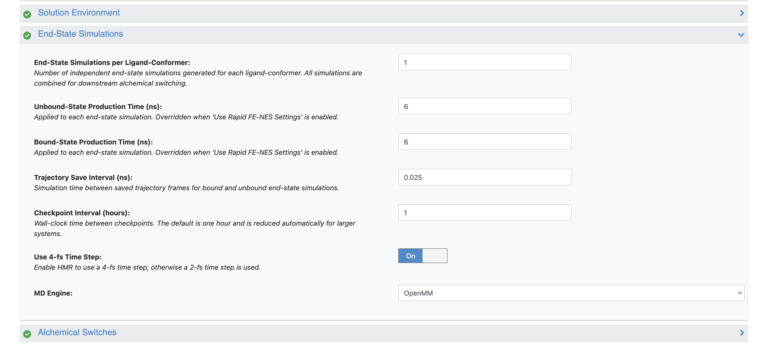
Figure 13. End-state simulation settings for the FE-NES for Binding Affinity Prediction Floe.

Each ligand can be asked to have more than one starting conformer for its equilibrium MD simulations. The number is applied identically to bound and unbound simulations. This is controlled by the End-State Simulations per Ligand-Conformer parameter, which is the first parameter in the End-State Simulations section (Figure 13). The default is 1.

The duration of bound and unbound state simulations can be set using the Bound State Production Time and Unbound State Production Time parameters. The default is 6 ns for both. If more than one conformer is set using the first parameter, then this duration set in these boxes is applied to each conformer. These are the second and third parameters in the End-State Simulations parameters (Figure 13).

Rapid FE-NES mode

When Rapid FE-NES mode is selected, these values are set to 1.5 ns for both bound and unbound simulations.

• Trajectory Save Interval (fourth parameter in Figure 13) sets the sampling interval during simulations. You can set the sampling interval to a value smaller than 0.025 ns to collect more frames from the equilibrium simulations. This will increase the size of the trajectory files but will also provide more information for offline analyses of trajectories.

• Checkpoint Interval (fifth parameter in Figure 13) controls the frequency of writing checkpoint files during the simulations. The value here largely pertains to the instances that become available for the simulations. If, however, the parameter is modified to a value greater than the default, fewer checkpoints will be saved. Likewise, for lesser values, more checkpoints will be saved. The latest checkpoint can be used to restart or recover simulations in case of any failures, using the Extend MD Simulations Floe.

• Use 4-fs Time Step (sixth parameter in Figure 13) controls the time step used for the MD simulations. If On (default), hydrogen mass repartitioning is applied to the system. If Off, the time step is set to 2 fs. The time step is applied to both bound and unbound simulations.

• MD Engine (seventh parameter in Figure 13) controls the MD engine used for the equilibrium MD simulations. All alchemical simulations are run using Gromacs.

Alchemical Switching Settings

The duration of the nonequilibrium switching simulations, number of switching simulations per edge, and time step used for the switching simulations can be set in the Alchemical Switching section.

The duration of each alchemical switch can be modified by changing Switching Time, and the number of switching simulations per edge can be modified by changing Switches per Edge.

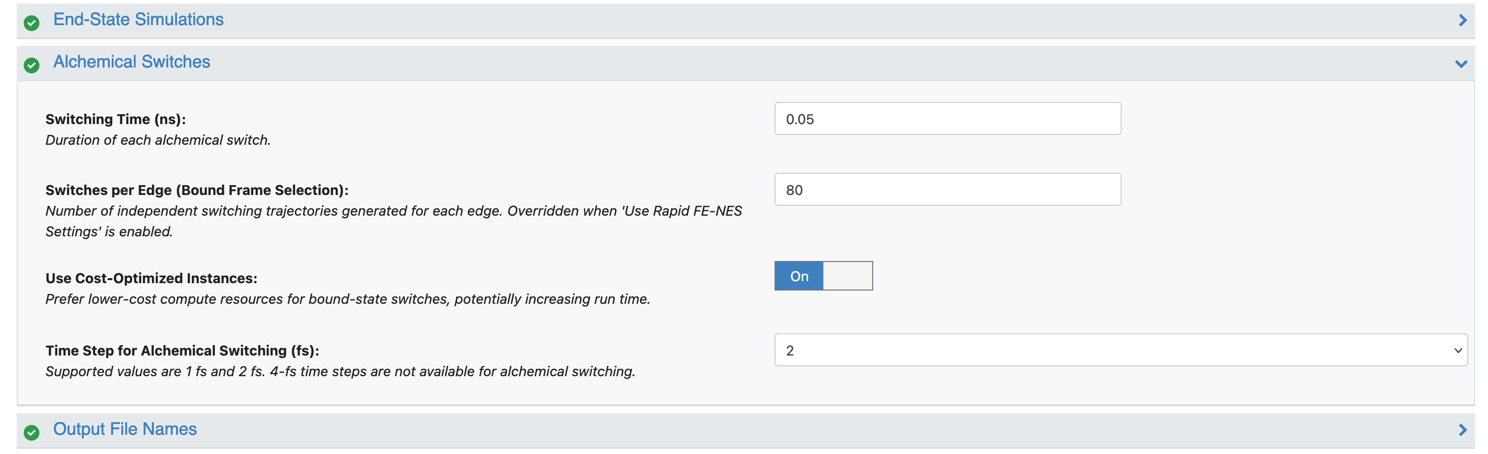
Figure 14. Alchemical switching settings for the FE-NES for Binding Affinity Prediction Floe.

Rapid FE-NES mode

When the Rapid FE-NES mode is selected, the number of switching simulations per edge is set to 20. The duration of the switching simulations and timestep values are unchanged: they are set to 50 ps and 2 fs, respectively.

Output File Names

The Output File Names section allows you to specify the names of the output files, datasets and Floe Reports generated by the floe. The default names are provided, but they can be changed as needed.

Advanced Compute Resources Settings

Several advanced compute resources settings can be modified in the Advanced Compute Resources section. These settings are intended for users with advanced knowledge of the Orion platform and are not required for most users. Left unchanged, the FE-NES for Binding Affinity Prediction Floe can generate predictions for up to 500 ligands (for a solvated system with up to 35K atoms) in a single run within 4 hours using the Rapid FE-NES mode.

Job Guardrails

Several guardrails are put in place to ensure that the floe can be run without the need for advanced knowledge of the Orion platform. These guardrails are intended to prevent users from making changes that could lead to failures due to insufficient compute resources or other issues.

Max Number of End-State Simulations

This guardrail limits the maximum number of end-state simulations that can be run in a single job. The default is 500, but it can be changed by the user.

Max Number of Alchemical Edges

This guardrail limits the maximum number of alchemical switches that can be run in a single job. The default is 1000, but it can be changed by the user.

Max Atoms Per Bound-State Simulation

This guardrail limits the maximum number of atoms that can be present in a bound-state simulation. The default is 250,000, but it can be changed by the user.

Under the Hood

Floe Architecture

The architecture of the floe can be found here.

The floe is composed of four main sections: Equilibrium Simulations, Edge Map construction, Nonequilibrium Switching, and NES Analysis for Affinity Prediction.

In the Equilibrium Simulations section, the floe runs equilibrium simulations for each ligand in the bound and unbound states. The bound state is simulated with the ligand in the binding site of the protein, while the unbound state is simulated with the ligand in solution. Force field parameters for these setups are applied using choices made in the floe parameters, and default values are provided for them.

Both bound and unbound equilibrium simulations are run for a default of 6 ns. For the bound state, the equilibrium simulations are preceded by an energy minimization step and a set of restrained NVT and NPT equilibration steps. Their durations are unchangeable. For the unbound state, an energy minimization step and an NPT equilibration step are run before the equilibrium simulations. Their durations are also unchangeable.

In the Edge Map Construction section, the floe constructs a map of edges between the ligands provided in the input dataset. Only those ligands that succeed in the equilibrium simulations are considered for edge construction. The edges are constructed based on the similarity of the ligands. Additionally, you can specify the type of edge map, with options for an OELOMAP, a STARMAP, or a STARMAP with two hubs (aka a Binary STARMAP). If a custom edge map is provided, the floe will skip the edge map construction step and use the provided edges for the RBFE calculations.

In the Nonequilibrium Switching section, the equilibrium runs used in a RBFE calculation are gathered, and frames are prepared for hybrid topology construction, which is also known as the Chimera molecule. Essentially, the ligands in an edge are topologically merged together with their force field parameters. They are then injected into selected equilibrium trajectory frames collected during the equilibrium runs. In the NES method, for each chimeric molecule (or edge), the following switching simulations are performed for each selected equilibrium frame:

1. Bound forward (ligA is mutated to ligB in the complex binding site)

2. Bound reverse (ligB is mutated to ligA in the complex binding site)

3. Unbound forward (ligA is mutated to ligB only in solution)

4. Unbound reverse (ligB is mutated to ligA only in solution)

By default, 80 equilibrium frames are selected for the bound and unbound runs (20 in Rapid FE-NES mode). Therefore, for each edge, a total of 320 switching mutations are completed (80 in Rapid FE-NES mode).

Switching mutations per edge

Regular FE-NES mode (80 frames per end-state run):

\[\begin{split}\begin{split} & 80~(\text{Bound forward}) \\ + & 80~(\text{Bound reverse}) \\ + & 80~(\text{Unbound forward}) \\ + & 80~(\text{Unbound reverse}) \\ = & ~320 \end{split}\end{split}\]

Rapid FE-NES mode (20 frames per end-state run):

\[\begin{split}\begin{split} & 20~(\text{Bound forward}) \\ + & 20~(\text{Bound reverse}) \\ + & 20~(\text{Unbound forward}) \\ + & 20~(\text{Unbound reverse}) \\ = & ~80 \end{split}\end{split}\]

Each alchemical switch starts with a short 5 ps NPT equilibration to adapt the equilibrium frame system to the new chimeric molecule, and is followed by a default 50 ps NPT ensemble simulation, where the chimeric molecule is switched between the starting and final ligand thermodynamic states. All runs use Gromacs as the MD engine at this stage.

The NES Analysis for Affinity Prediction section analyzes the NES data to produce binding affinities and relative binding affinity results. For each edge, the forward and reverse functions for the bound and unbound switching are compared by using the BAR method. These values are used to compute the \(\Delta G_{Bound}\) and \(\Delta G_{Unbound}\) free energies that are related to \(\Delta\Delta G\). The RBFE value of an edge is used to estimate the affinity values by using the maximum likelihood estimator.

Additional Resources

The following sections provide further details on the FE-NES for Binding Affinity Prediction Floe:

• FE-NES theory: Background on the nonequilibrium switching method used to compute relative binding free energies.

• FE-NES Workflow Diagram: Overview of the workflow stages, from system preparation to RBFE prediction.

• Experimental Affinity Inputs: Instructions for providing experimental affinities from a dataset or a text file.

  • Experimental Affinity Provided by a Text File: Syntax and delimiters for the experimental affinities text file.

  • Affinity Conversion Table: Formulas used to convert experimental affinities to kcal/mol.

• Downloading Trajectories from Floe Reports: Instructions for downloading MD trajectories from the Trajectory Downloader Floe Report page and converting them for offline analysis.