Theory
A Model of Multiple Models
Model Descriptors
Machine Learning Methods
3D Conformer Generation
Applicability Domain and Prediction Confidence
Model Interpretation
A Model of Multiple Models
The 3D model developed in this work is a model of multiple models, sometimes referred to as the consensus or the COMBO model. The prediction from the consensus model is provided as the median of the individual model predictions; the prediction confidence is also obtained as the median of the individual model confidences.
Four individual 3D models are currently built with various combinations of descriptors and machine learning methods. The names of the individual models consist of both the descriptor types and the machine learning methods used. The four individual models currently built are ROCS-kPLS, EON-kPLS, ROCS-GPR, and EON-GPR. 2D-GPR is used as the baseline/null model. Figure 1 illustrates the 3D and 2D models built in this work.
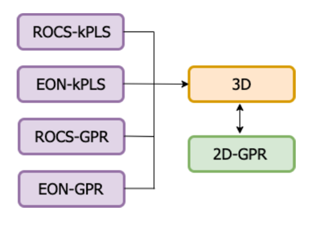
Figure 1. Chart of the models built in this work.
Model Descriptors
3D molecular similarity as described by ROCS®, with shape and color, has been a tremendous success for virtual screening. Here shape- and color-based similarities are used as ROCS descriptors. A more rigorous description of similarity can be provided by EON descriptors, where color is replaced by electrostatic potential similarity. EON-based descriptors are also exploited here as an alternative to ROCS descriptors. Besides the ROCS- and EON-based similarity descriptors, 2D circular fingerprint (FP) based similarity is also included in some of the individual 3D models. Table 1 lists the descriptors used in the four individual 3D models.
Model Name |
Descriptors |
|---|---|
ROCS-GPR |
FP Tanimoto + ROCS Tanimoto combo (shape + color) |
EON-GPR |
FP Tanimoto + EON Tanimoto combo (shape + electrostatics potential) |
ROCS-kPLS |
Shape overlap + constant*color score |
EON-kPLS |
Shape overlap + constant*electrostatic potential overlap |
In Table 1, “constant” for the kPLS models is a normalization factor determined using the maximum self overlap of the training set. Besides the four 3D models, a 2D-GPR model using the FP Tanimoto as descriptors is also built as a baseline/null model. In practice, the descriptor, or feature vector of a molecule, is generated by calculating the pairwise Tanimoto or overlap against each of the molecules in the training set.
Machine Learning Methods
Two distinct machine learning approaches, namely kernel Partial Least Squares (kPLS) and Gaussian Process Regression (GPR), are used for model building. These traditional machine learning methods are more suitable for building models with small datasets, which is the case for potency models.
Gaussian Process Regression (GPR)
Gaussian Process Regression (GPR) is a nonparametric, Bayesian supervised machine learning method. GPR learns using a Bayesian approach by inferring a probability distribution over all possible values, instead of learning an exact value for each parameter. GPR works well with small datasets. Predictions made by GPR are probabilistic (Gaussian).
The GPR methods as implemented in the scikit-learn package ([Pedregosa-2011]) are used directly.
A combination of the WhiteKernel, DotProduct, and RBF kernel are used as the GPR Kernels.
Kernel Partial Least Squares (kPLS)
Partial Least Squares (PLS) regression is an excellent tool for making predictive models when the feature space is larger than the number of training set points and when the features are highly correlated. It is a latent variable approach that tries to find the multidimensional direction in the feature vector space (\({X}\)) that explains the maximum multidimensional variance direction in the predicted variable space (\({Y}\)). In what follows, \({n}\) will be used to denote the number of examples and \({m}\) the number of features. In a typical 3D-QSAR model, \({n}\) would be the number of molecules and \({m}\) the number of descriptors, or length of the feature vector.
When the feature space becomes exceptionally large, a suitable kernel operation can be incorporated to simplify the mathematical operations. The idea behind kernel PLS (kPLS) is to replace matrix operations of size \({n \times m}\) with compact ones \({n \times n}\), which is the inner product between feature vectors. In terms of shape- based similarity, the dot product essentially refers to the overlap between two molecules.
The number of latent variables controls the amount of training set information that is embedded into the model. The number of latent variables is thus a hyperparameter for the model that must be optimized, to avoid either undertraining or overtraining of the model. We use a leave-one-out or 50-fold random split cross-validation to optimize this hyperparameter.
One of the attractive features of kPLS is that it provides a physical and interpretable model, instead of a complex black-box-like model as obtained from GPR or other advanced machine learning models. The final prediction model takes the form
where \({B}\) represents the column vector of regression coefficients, \({s}\) the column vector of pairwise descriptors, and \({B_0}\) a scalar constant.
Note
To train a kPLS model, the descriptors cannot be arbitrary and need to be pairwise descriptors.
3D Conformer Generation
High quality 3D conformers are essential for generating quality 3D-QSAR descriptors. The crystallographic pose conformers should be used directly for model building, when available.
Posit is utilized for ligand pose generation, when a crystallographic structure of the target is available. Posit utilized in this package mostly follows the Posit algorithm under OEDocking TK as implemented, except for an extension for handling molecules with unspecified stereo (described below). Besides being the best-in-class pose prediction method, Posit also provides confidence estimates in the form of Posit probability, as a measure of quality on the predicted pose, which could be exploited in providing confidence on model predictions.
FlexiROCS™ is the choice for conformer generation when building models in a ligand-based setting. FlexiROCS uses the same technology as used in the ShapeFit method from OEDocking TK, except for bump checking against the target receptor. Similar to Posit, FlexiROCS also provides confidence on the quality of the predicted conformers.
Stereoisomer Handling
When molecules with unspecified stereo are provided, molecules are first enumerated for all stereo variants before conformer generation. The best conformer for each of the variants is obtained, followed by picking the one with the best corresponding score.
Applicability Domain and Prediction Confidence
Applicability models for the individual models, including 2D, are developed based on minimum dissimilarity to the training set. The minimum dissimilarity of a molecule \({i}\) to a training set of size \({N}\) can be expressed as
Here \(\max_{1\le j \le N} S_{ij}\) is the maximum Tanimoto of molecule \({i}\) to the training set molecules. \({S_{max}}\) is the upper bound of the Tanimoto, or normalization factor, depending on the model (1.0 for 2D-GPR models, 2.0 for 3D kPLS models, and 3.0 for 3D GPR models). In other words, the minimum dissimilarity is equivalent to 1.0 – normalized maximum similarity.
Global applicability models are trained for all individual 3D and 2D models using experiments where molecules on the validation set exhibit various degrees of dissimilarity with the training set. Datasets with crystallographic poses and experimental binding affinity data were curated from the RCSB website for nine different targets. Experiments were performed by doing cluster and random splits from these nine datasets. The fraction of accurate results corresponding to any given dissimilarity was first estimated based on Figure 2 below, which was later converted to a corresponding prediction confidence. A prediction is deemed accurate if it is within one log unit from the experimental value.
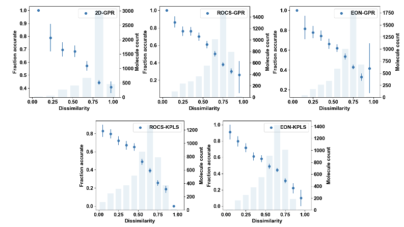
Figure 2. Fraction accurate vs. minimum dissimilarity to training set obtained from all experiments.
Note
Here, prediction confidence can be understood as the probability of a prediction to be accurate (within 1 log unit of experimental value).
For conformers generated by Posit or FlexiROCS, prediction confidence is estimated by multiplying the applicability confidence by the pose confidence (i.e., a product of two probabilities). For a crystallographic pose or for a pose prediction method that does not have an associated confidence, the pose confidence is taken to be 1.0.
Model Interpretation
Due to the nature of the kPLS algorithm, it can be used to make predictions for fragments of a molecule. This feature of kPLS can be exploited to generate model interpretation, aiming to explain the areas in the active site where the presence of a specific type of functional group can improve the potency of molecules.
To generate model interpretation, the active site domain is determined first by encapsulating the volume containing all of the molecules in the training set. A grid is generated on the active site domain, and the potency scores of different types of probe particles are predicted on the individual grid points.
For a specific probe type, a high surface is obtained from the part of the grid that gives the top 2% of the highest predicted positive scores, indicating locations where the presence of such probe particles is favorable. Similarly, a low surface is obtained from the part of the grid that gives the bottom 2% of the lowest predicted negative scores, indicating locations where the presence of such probe particles is unfavorable.