Tutorials
The OpenEye Cryptic Pocket Detection Floes aim to explore ligand binding sites and help with assessing the drugability of difficult protein targets. It does this by enabling the preparation and running of Weighted Ensemble (WE) Molecular Dynamics (MD) simulations to subsequently identify potential cryptic pockets sites given the enhanced conformational sampling. The use-cases for this package include but are not limited to:
Proteins that exhibit smooth surfaces with no visible pockets where we might want to see if a cavity could open.
Proteins where the known pockets are not desirable candidates for drug development. This package can be used to reveal other potential binding pocket sites. For example, the GDP/GTP binding pockets of Ras proteins are a known binding pocket, but due to the pocket similarities across multiple families of K-Ras proteins and the binding affinity for GDP/GTP, it is not an ideal candidate for developing a drug.
When successful, this package enables the use of other OpenEye discovery tools.
Note
This package operates under the assumption that the normal mode progress coordinates will help to sample the ensemble of conformations. The normal modes that are chosen determine the part of the conformation ensemble that is enhanced and a different selection of normal modes could reveal a different pocket opening.
If you are not pleased with the outcome of the C1 and C2 simulations, you might consider:
Extending the simulation and re-running the analysis. In the case of mixed-solvent simulations, longer simulations increase the chance of seeing exposon binding.
Revisiting the A3a floe and choosing a different set of normal modes to enhance the sampling of a different conformation ensemble accessible through those modes.
Warning
This package has been intentionally split into a total of 12 floes. You will run 8-9 floes (depending on whether extending the simulation with the A3b Floe is required/desired) in order to sample and analyze a protein. This decision was made because there are a number of potential failure points where, upon reviewing the results, a user might need to re-run a floe or two until they are satisfied with the results. The complexity of the problem that this package aims to address means that these floes may take longer to learn than the average floe. At the start of each tutorial, we give an estimate of the time and cost required to run each of the floes.
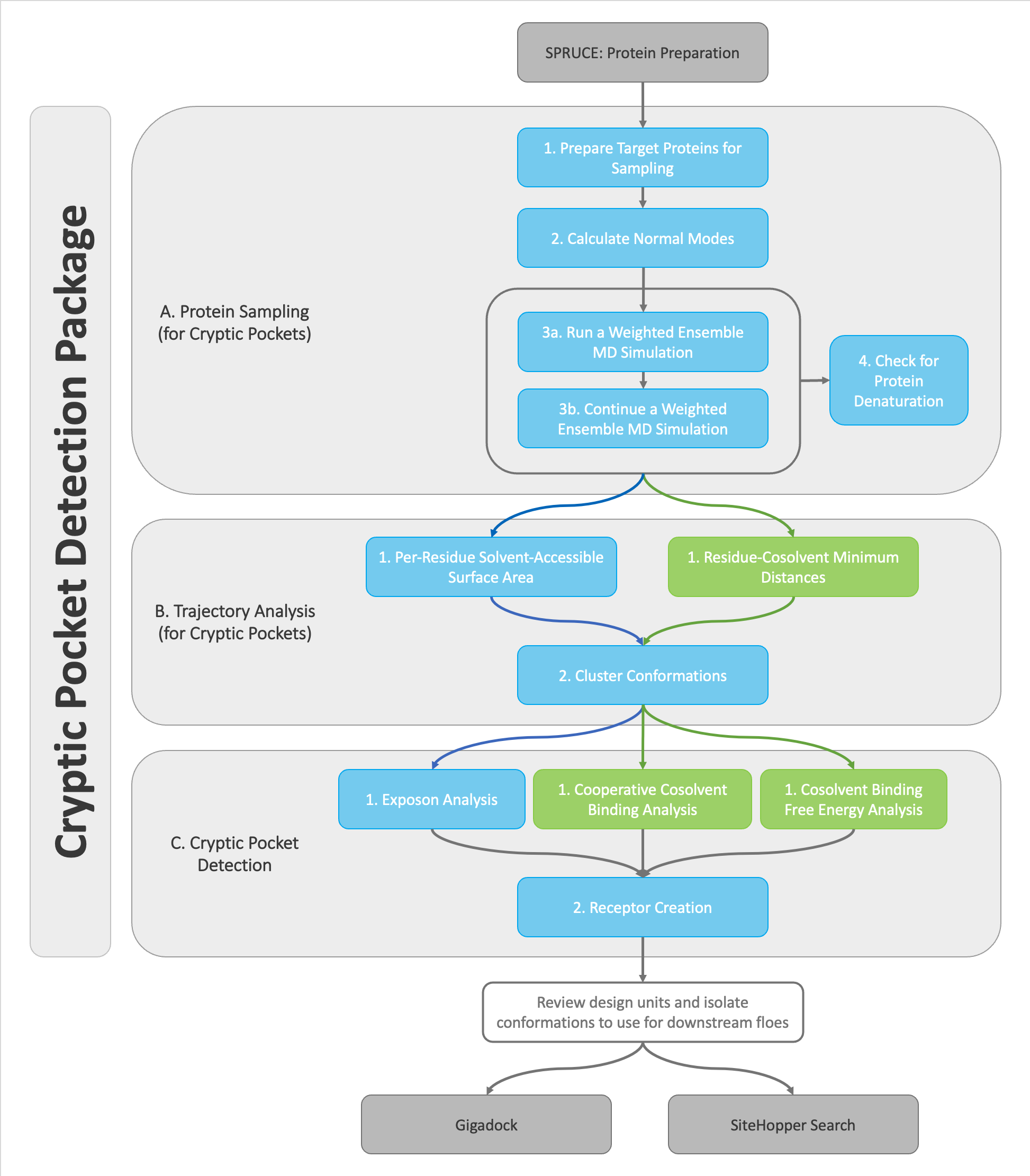
Decision tree for the OpenEye Cryptic Pocket Detection floes. If the protein sampling simulations are solvated in water, the only options for analysis follow the blue arrows and blue floes. If the protein sampling simulations are solvated in water and xenon, any of the analyses are viable.
There are four distinct combinations of the floe options that are possible. The decision tree is shown in the figure above. Your first decision point will be choosing weather to solvate your target protein in water (TIP3P) alone or to solvate in a water and xenon mixture in the A1. Protein Sampling (for Cryptic Pockets): Solvate and Equilibrate Target Protein Floe. In this tutorial, these two solvent environments will be referred to as single-solvent and mixed-solvent, respectively.
At this stage, if you choose to run a single-solvent simulation, you will run a single set of floes, including the per-residue solvent accessible surface area (SASA) analysis and exposon analysis to detect cryptic pockets. The blue path in the figure above guides you through the floes in blue boxes that you will run for this option. If this is your cup of tea, proceed to the single-solvent exposon tutorial when you are ready.
If you choose to run a mixed-solvent simulation, you will reach a second decision point when running the B1. Trajectory Analysis (for Cryptic Pockets) floes. You have two choices; you can perform a per-residue SASA analysis or a residue-cosolvent minimum distance analysis. If you choose the first option, you will again end up with only one option in the C1 floes to run exposon analysis (mixed-solvent exposon tutorial). If you choose to perform the residue-cosolvent minimum distance analysis, your last decision point will be when running the C1. Cryptic Pocket Detection floes. You will have the choice to run the cooperative cosolvent binding (CCB) analysis (mixed-solvent CCB tutorial) or the cosolvent binding free energy (CBFE) analysis (mixed-solvent CBFE tutorial).
Warning
In summary, there are two B1 floes and three C1 floes. These floes are branching points in the sequence of floes that you will be running. Depending on which of the B1 floes is chosen, you will limit which of the C1 floes you have to chose from. Select the tutorial that will guide you through using the set of B1 and C1 floes that you are interested in.
When running the tutorial, be careful to select the right B1 and C1 floe!
This is a comprehensive list of the floes in this package:
- Protein Sampling (for Cryptic Pockets)
A1. Protein Sampling (for Cryptic Pockets): Solvate and Equilibrate Target Protein from the OpenEye Cryptic Pocket Detection Floes package.
A2. Protein Sampling (for Cryptic Pockets): Calculate Normal Modes from the OpenEye Cryptic Pocket Detection Floes package.
A3a. Protein Sampling (for Cryptic Pockets): Run a Weighted Ensemble MD Simulation from the OpenEye Cryptic Pocket Detection Floes package.
A3b. Protein Sampling (for Cryptic Pockets): Continue a Weighted Ensemble MD Simulation from the OpenEye Cryptic Pocket Detection Floes package.
A4. Protein Sampling (for Cryptic Pockets): Check for Protein Denaturation from the OpenEye Cryptic Pocket Detection Floes package.
- Trajectory Analysis (for Cryptic Pockets)
B1. Trajectory Analysis (for Cryptic Pockets): Per-Residue SASA from the OpenEye Cryptic Pocket Detection Floes package.
B1. Trajectory Analysis (for Cryptic Pockets): Residue-Cosolvent Distances from the OpenEye Cryptic Pocket Detection Floes package.
B2. Trajectory Analysis (for Cryptic Pockets): Cluster Conformations from the OpenEye Cryptic Pocket Detection Floes package.
- Cryptic Pocket Detection
C1. Cryptic Pocket Detection: Exposon Analysis from the OpenEye Cryptic Pocket Detection Floes package.
C1. Cryptic Pocket Detection: Cooperative Cosolvent Binding Analysis from the OpenEye Cryptic Pocket Detection Floes package.
C1. Cryptic Pocket Detection: Cosolvent Binding Free Energy Analysis from the OpenEye Cryptic Pocket Detection Floes package.
C2. Cryptic Pocket Detection: Receptor Creation from the OpenEye Cryptic Pocket Detection Floes package.
Warning
Before starting the tutorials, make sure that your stack has a project space for running the tutorials in. See the instructions in the Creating an Orion Project (Optional) tutorial. Given the expense of running Weighted Ensemble simulations, we recommend that a full simulation dataset and collection should only be generated once for the mixed-solvent and single-solvent preparation, and then shared with others. This first full simulation will also allow others taking the tutorial to skip ahead in the tutorial steps to the Trajectory Analysis (for Cryptic Pockets) Floes.
Contents:
- Creating an Orion Project (Optional)
- Design Unit Preparation for Beta-Lactamase (Optional)
- Cryptic Pocket Detection Tutorial: Exposons Analysis of Beta-lactamase (single-solvent)
- Cryptic Pocket Detection Tutorial: Exposons Analysis of Beta-lactamase (mixed-solvent)
- Cryptic Pocket Detection Tutorial: Cosolvent Binding Free Energy Analysis of Beta-lactamase (mixed-solvent)
- Cryptic Pocket Detection Tutorial: Cooperative Cosolvent Binding Analysis of Beta-Lactamase (mixed-solvent)