Cryptic Pocket Detection Tutorial: Cosolvent Binding Free Energy Analysis of Beta-lactamase (mixed-solvent)

In this tutorial, we will guide you through the process of using the Cryptic Pocket Detection package to identify pockets on beta-lactamase using cosolvent binding free energy analysis of a mixed-solvent (TIP3P water and Xenon) simulation. Cosolvent binding free energy analysis can only be performed on mixed-solvent simulations.

Tip

The Protein Sampling (for Cryptic Pockets) only has to be run once to generate the data for the mixed solvent simulations. If you or someone else on your stack has already generated the data for this, you can skip to the Trajectory Analysis (for Cryptic Pockets) part of the tutorial. It should be noted that the process of running the Protein Sampling (for Cryptic Pockets) Floes (A1 - A4) are very similar for mixed and single solvent simulations. If you have also already run the Cooperative Cosolvent Binding tutorial, you can skip to the Cryptic Pocket Detection part of the tutorial.

In the figure below, each of the colored boxes (blue/green) represent floes that this tutorial will guide you through. The greyed-out floes represent alternative paths that could be taken to identify cryptic pockets that are explained in other tutorials.

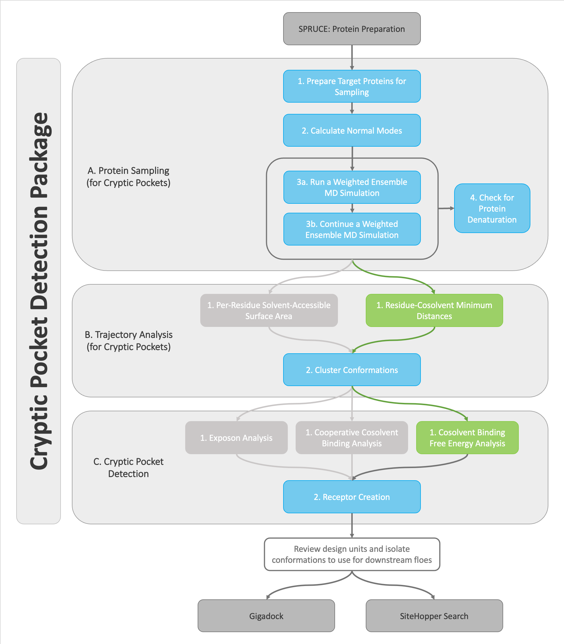
Decision tree for the OpenEye Cryptic Pocket Detection floes. This tutorial demonstrates how to use the highlighted floes in the decision tree.

Protein Sampling Cost and Run Time Estimates

Floe Name	Time (hrs)	Cost ($)
SPRUCE: Protein Preparation	0:12	0.21
Subset Design Unit	0:03	0.03
A1. Protein Sampling (for Cryptic Pockets): Solvate and Equilibrate Target Protein	1:25	3.24
A2. Protein Sampling (for Cryptic Pockets): Calculate Normal Modes	0:08	0.05
A3a. Protein Sampling (for Cryptic Pockets): Run a Weighted Ensembled MD Simulation (48 iteration)	13:02	154.09
A3b. Protein Sampling (for Cryptic Pockets): Continue a Weighted Ensembled MD Simulation (2 iteration)	0:34	6.12
A3a. (5 iteration)	1:05	5.90
A3b. (5 iterations)	1:08	10.35
A4. Protein Sampling (for Cryptic Pockets): Check Protein Denaturation	0:52	15.26
Total (50 iterations - first run)	16:16	179.00
Total (10 iterations - subsequent runs)	4:53	35.04

Pocket Detection Cost and Run Time Estimates

Floe Name	Time (hrs)	Cost ($)
B1. Trajectory Analysis (for Cryptic Pockets): Residue-Cosolvent Minimum Distances	2:30	6.00
B2. Trajectory Analysis (for Cryptic Pockets): Cluster Conformations	9:00	27.00
C1. Cryptic Pocket Detection: Cosolvent Binding Free Energy Analysis	3:00	30.00
C2. Cryptic Pocket Detection: Receptor Creation	3:00	4.00
Total (50 iteration simulation)	17:30	67.00

To begin this tutorial, download the prepared design unit for the 1JWP protein structure of beta-lactamase:

Beta-Lactamase 1JWP protein structure DU

For an example of how to prepare the apo 1JWP protein structure design unit, see the Design Unit Preparation for Beta-Lactamase (Optional) tutorial.

Protein Sampling (for Cryptic Pockets)

Solvate and Equilibrate Target Protein (Mixed Solvent)

In this section, we will show you how to use the SPRUCE prepared beta-lactamase protein in an MD preparation floe A1. Protein Sampling (for Cryptic Pockets): Solvate and Equilibrate Target Protein.

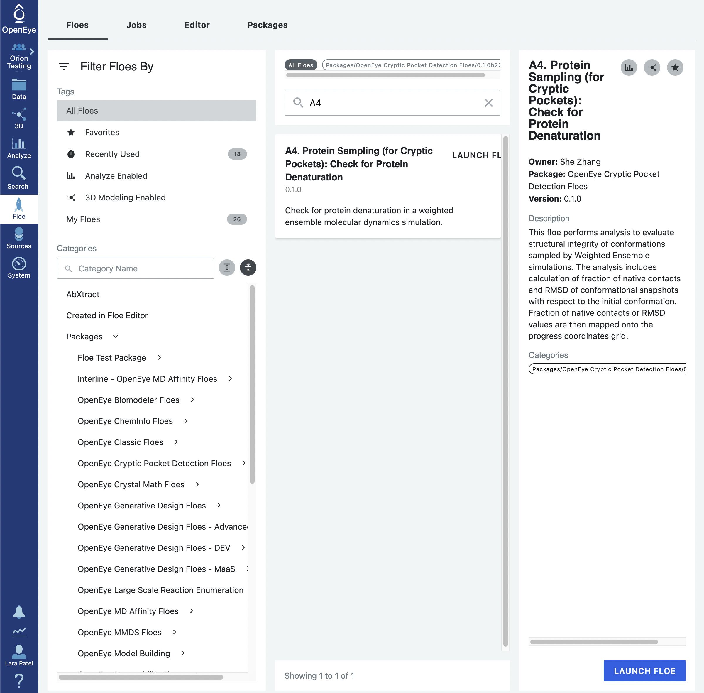
Start by using the left hand vertical navigation tabs to go to Floes. Under the horizontal Floes tab, you will search for the floe that we will Start by using the left hand vertical navigation tabs to go to Floe. Under the horizontal Floes tab, you will search for the floe that we will be using. You can use the search function or you can use the left side options to search for the package itself. Click on Packages to expand the list of packages and click on the OpenEye Cryptic Pocket Detection Floes package.

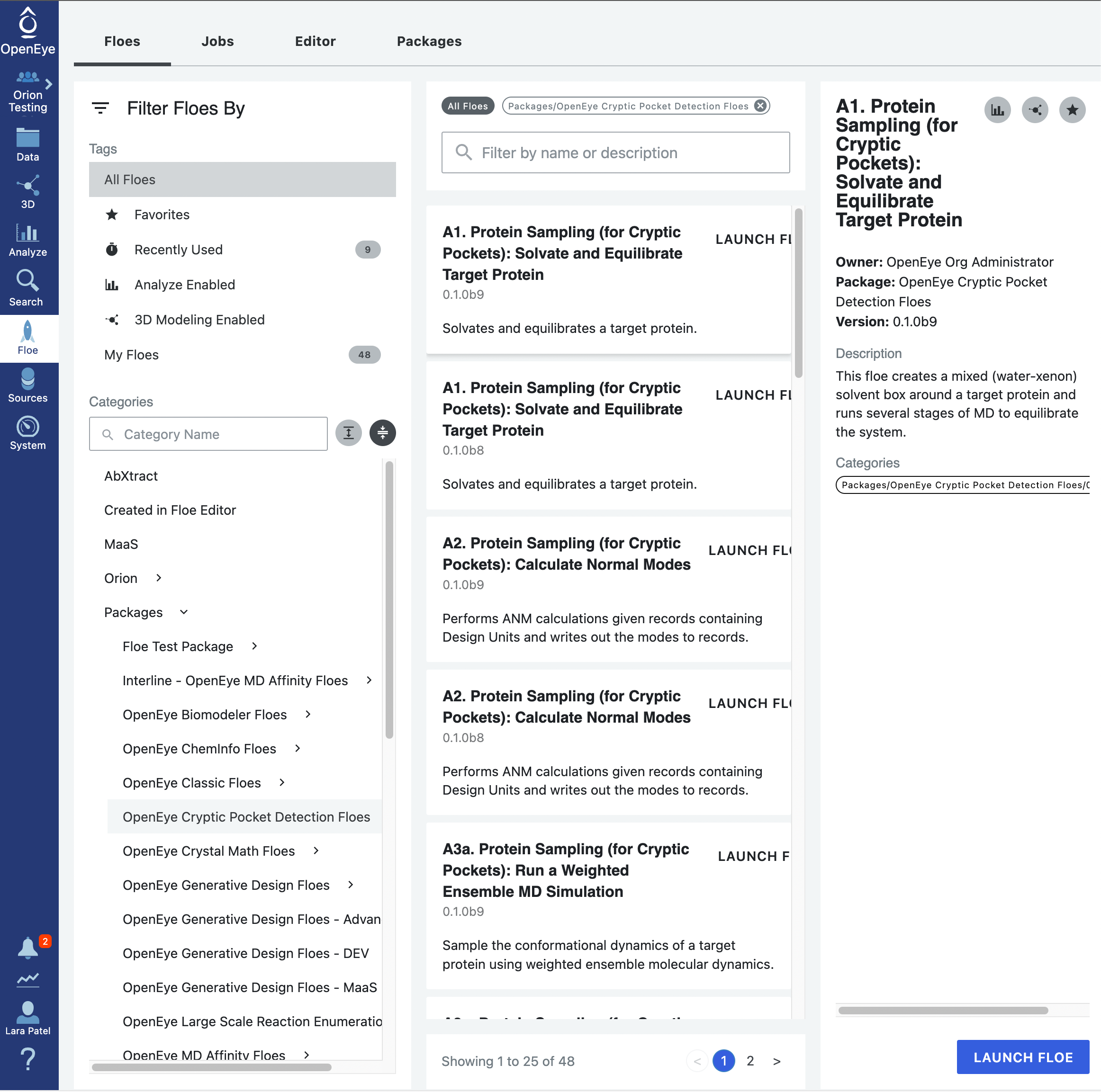
This will ensure that the floes listed in the middle of the page are from the Cryptic Pocket Detection package. The floes are listed in the order that they will be run. Click on the first floe, A1. Protein Sampling (for Cryptic Pockets): Solvate and Equilibrate Target Protein, and then click on the blue LAUNCH FLOE button in the bottom right corner of the page.

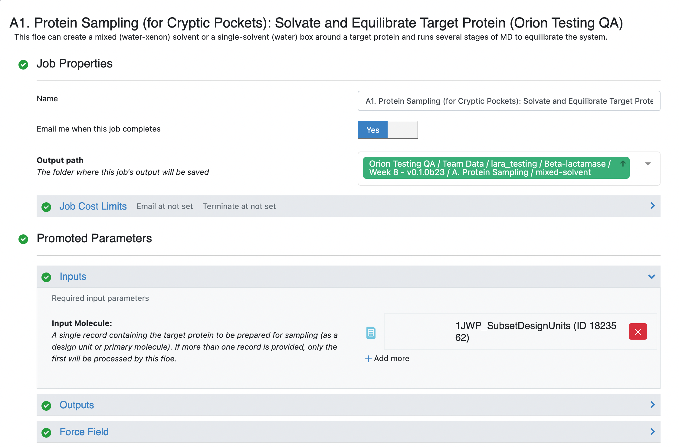
On the page that opens, select the place where your output data will be directed by specifying the Output Path, choose the Input Molecule to be the SPRUCE prepared dataset for beta-lactamase. You can customize the output dataset and collection names under the Outputs options. We will be running a mixed-solvent simulation. This is compatible with all of the analysis options in the cryptic pocket detection package and is therefore the most versatile option. We will be using the default Molar fractions and Solvents in this tutorial. You may add a 150 mM Salt Concentration to the solvation box. For those who are hesitant to use a cosolvent, we provide a separate tutorial for preparing single-solvent simulation systems here but this will limit you to exposons analysis during cryptic pocket detection.

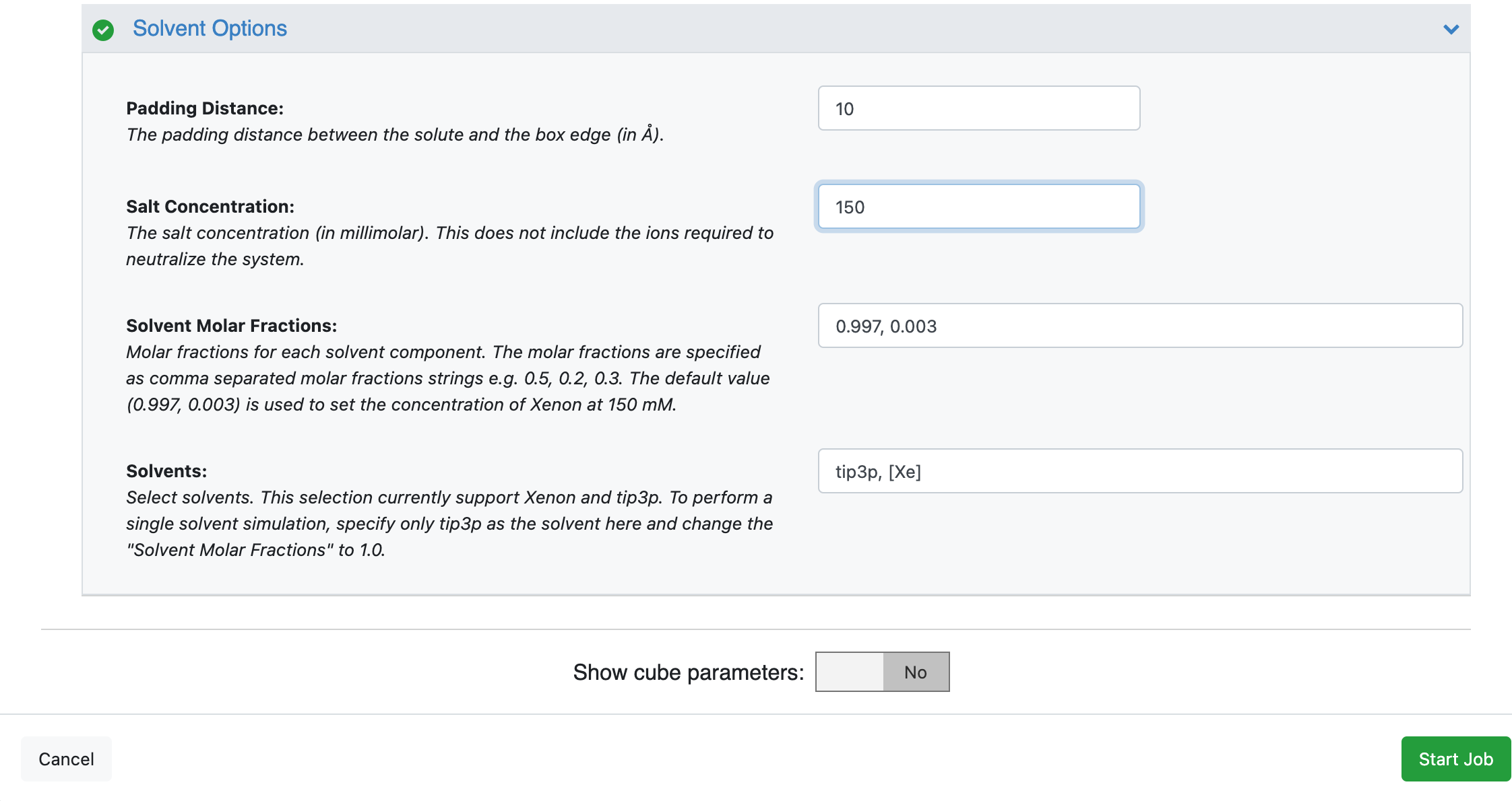
Click on the green Start Job button a the bottom right corner of the page.

Tip

Wait for the submitted job to finish. This should take approximately one hour.

If the job completed successfully, there should be four outputs in total: an MD dataset, a reference PDB file containing all of the system components, an h5.tar.gz file, and a collection.

Calculate Normal Modes

Normal modes are orthogonal degrees of motion that the protein can access. Typically, the modes with lower frequencies tend to describe collective motions that engage large parts of the protein; therefore, they are referred to as the global modes [Bahar2010]. The modes are modeled based on the input PDB structure that has been relaxed using the A1. Protein Sampling (for Cryptic Pockets): Solvate and Equilibrate Target Protein Floe. As such, your global modes may not look exactly like the ones displayed in this tutorial, since your protein relaxation will have resulted in a slightly different structure.

Global modes are used as progress coordinates to drive sampling of a chosen protein. Larger changes in protein backbone motions occur on timescales that are expensive to sample via brute force simulation. The hope is that by using global modes to drive the larger protein fluctuations, we can sample a broad range of conformations including those that reveal pocket opening. This tutorial demonstrates how to identify global modes from normal modes calculated using the input structure.

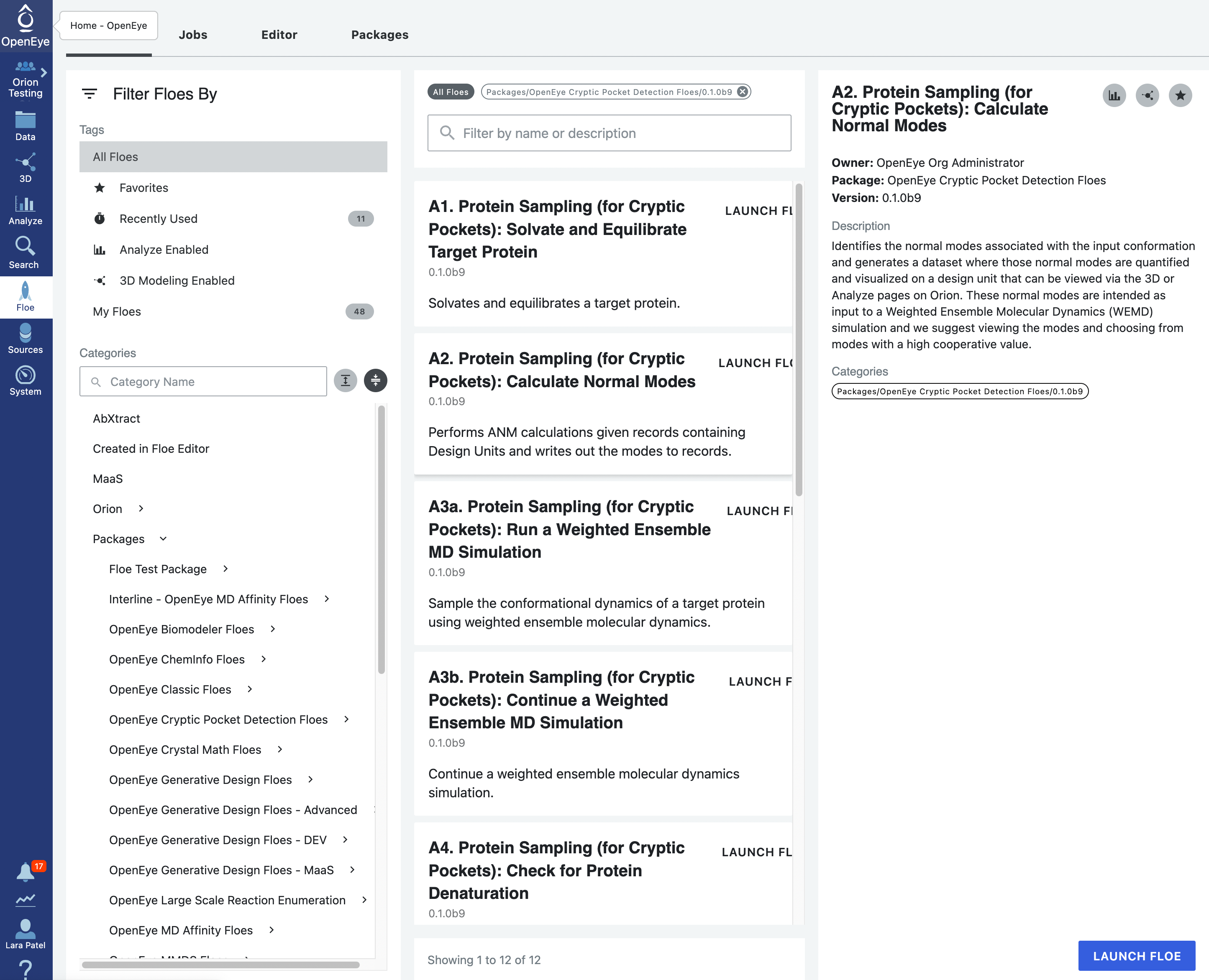
Start by clicking on the blue navigation side bar Floe tab. Click on the Floes tab at the top of the page and then filter for Packages -> OpenEye Cryptic Pocket Detection Floes. Select the A2. Protein Sampling (for Cryptic Pockets): Calculate Normal Modes Floe and click the LAUNCH FLOE button.

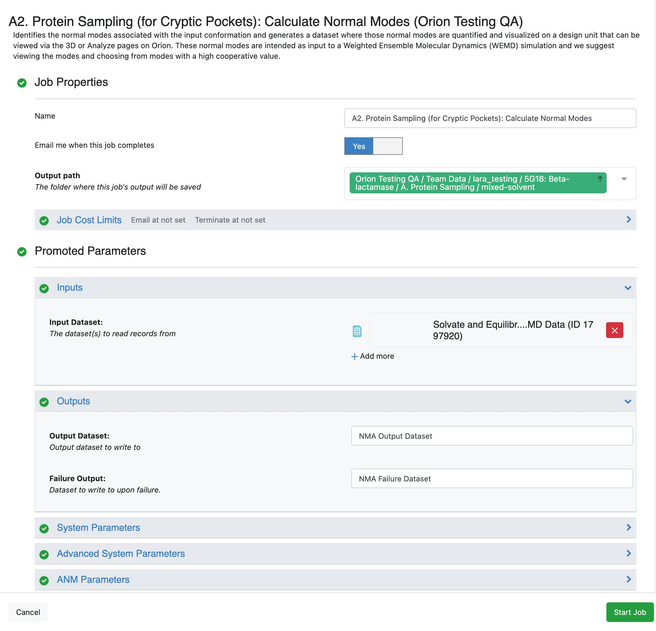
This opens up the floe options page, and you will want to customize the Output Path and Output options. You will also need to select the output MD Data dataset record from the A1. Protein Sampling (for Cryptic Pockets): Solvate and Equilibrate Target Protein Floe. Click the Start Job button.

Tip

Wait for the submitted job to finish. This floe typically takes less than five minutes to run, just enough time to get a cup of tea or coffee.

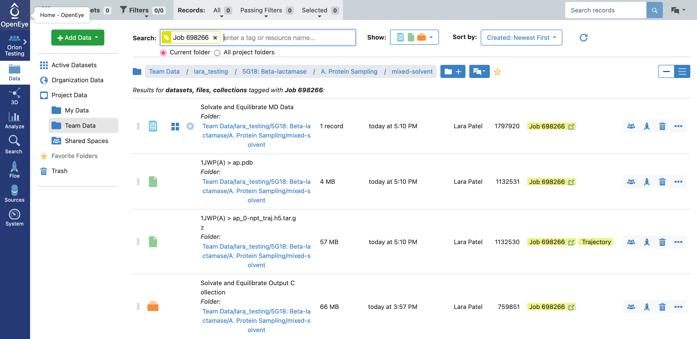
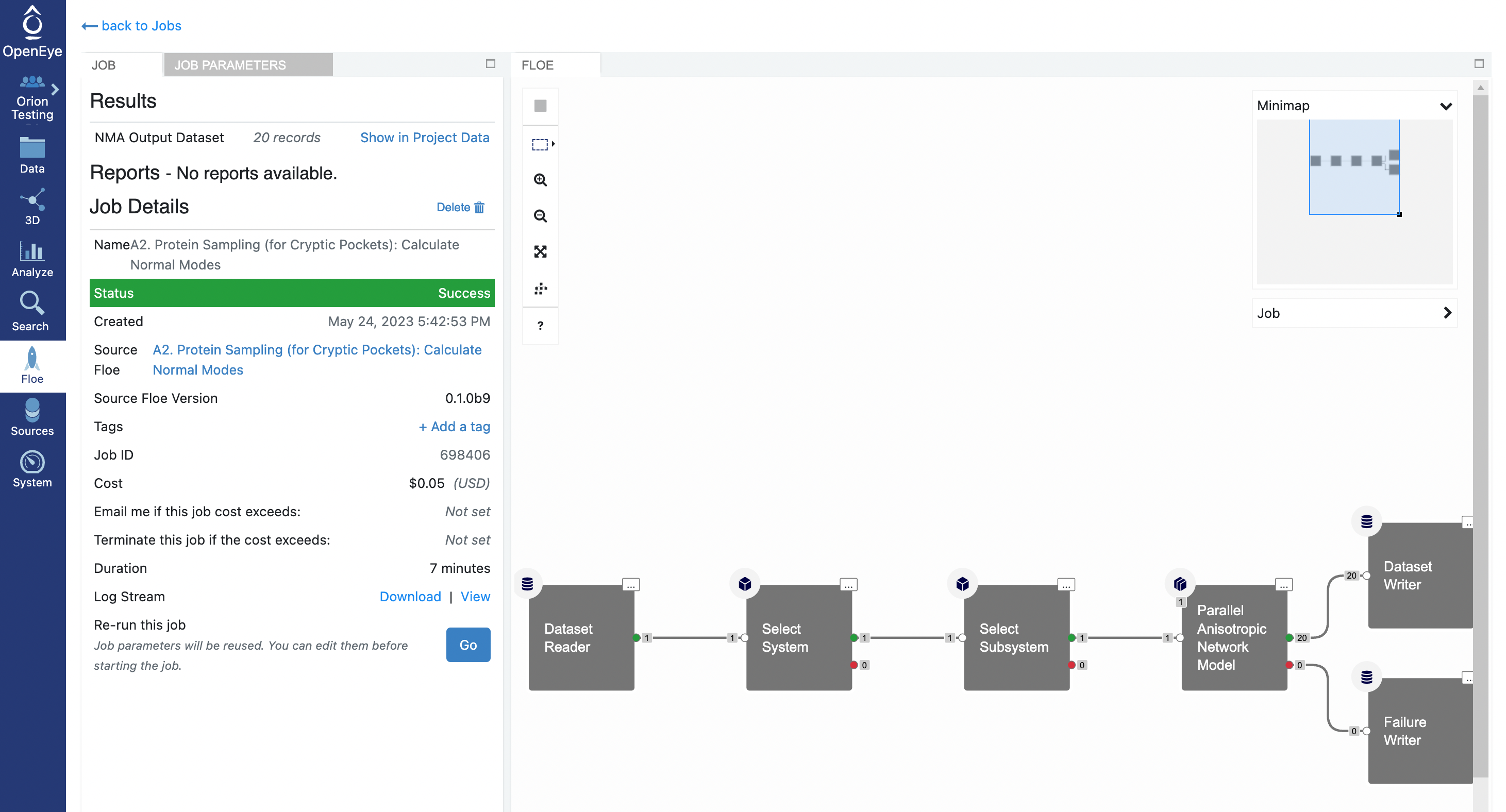
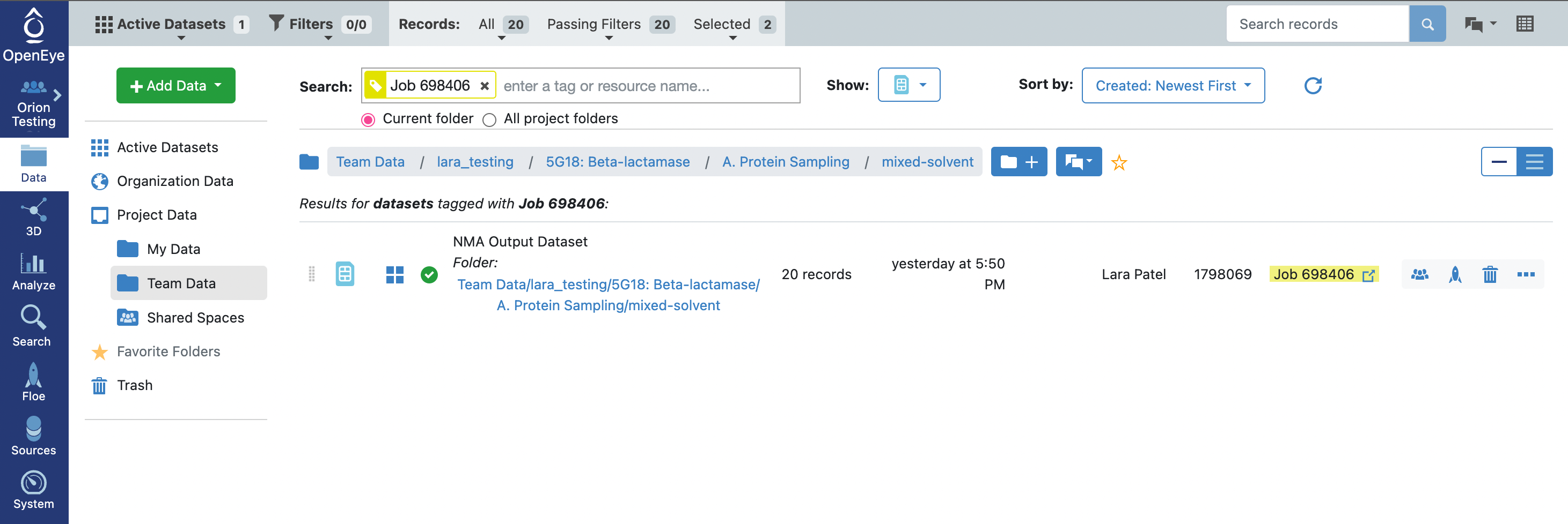
When the floe job is complete, the output normal mode analysis dataset should be inspected using the Analyze page to identify the best normal modes to use in the next floe. You can get to the dataset by clicking on the normal mode analysis job. Click on the Floe tab on the blue navigation side bar and then click on the Jobs tab at the top of the page. Then click on the job that you want to inspect. Under Results, click on Show in Project Data to see the dataset associated with the job.

This will redirect you to the Data navigation side bar tab and show only the dataset associated with the job. Click on the icon of a blue circle with a + symbol that is next to the dataset name. It will change to a green circle with a white checkmark and will allow you to view the dataset in the 3D Modeling page and the Analyze page.

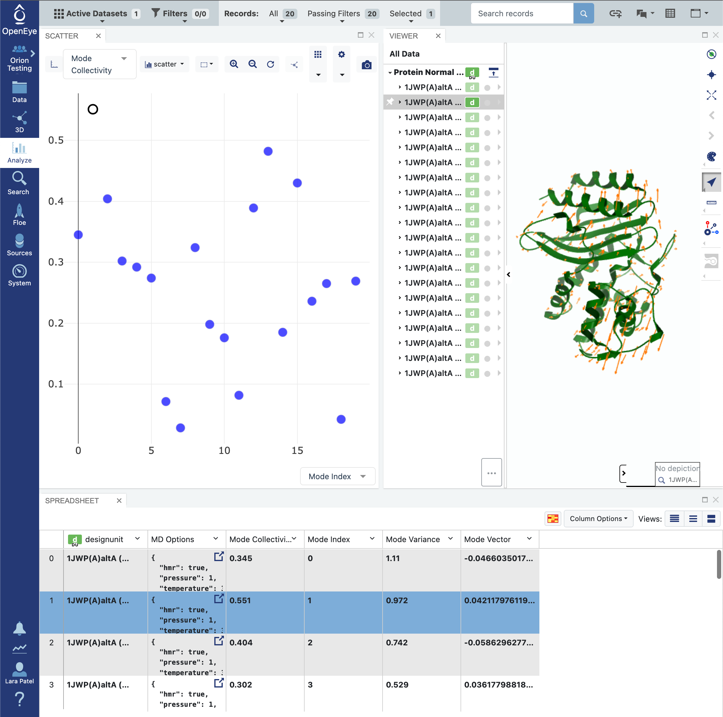
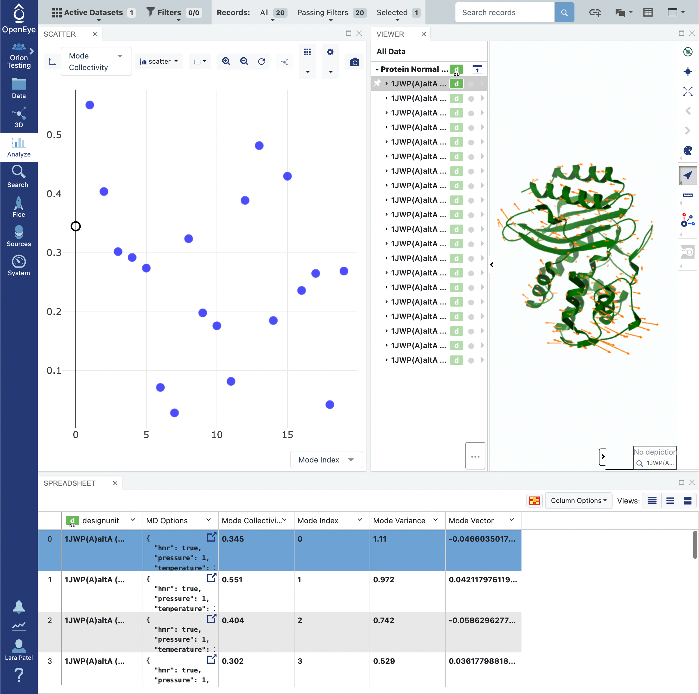
Click on the blue navigation side bar Analyze tab. Make sure that the Active Dataset is set to the normal mode analysis dataset. On the scatter plot on the Analyze page, use the Mode Index for the x-axis and use the Mode Collectivity for the y-axis. Also click on the Layouts button in the top-right corner and select the Analyze with 3D option. This shows a visual representation of the mode vectors as orange arrows on a representative structure of the protein taken from the solvated and relaxed protein structure supplied for the normal mode analysis.

Mode indices are assigned to the modes ranking them from the lowest frequency modes to the highest. By default, only the top 20 (out of thousands) modes are calculated. As mentioned above, modes with the lowest frequency, or equivalently, the highest magnitude, tend to describe global motion. However, low frequency modes may also correspond to modes where free loops or trailing protein tails dominate the normal mode. This is called the “tip effect”. To avoid issues caused by the tip effect, we recommend picking the modes with high Mode Collectivity among the top 20 modes using the graph mentioned above.

The tip effect can also be avoided by selecting a subset of residues on the protein that exclude loops and/or portions of the protein that you know will dominate the normal modes. In the floe, this can be done by specifying the range(s) of residues that are considered as part of the system, excluding the tail region, using the System Parameters -> String Selection parameter. The general syntax follows

[chain_id]:[from_res_num]~[to_res_num]

In practice this would look like A:1~150 when selecting residue numbers 1 to 150 on chain A of the input protein. Omitting either from_res_num or to_res_num allows for open-ended selections. For example, A:10~ can be used to select any residue with a residue number greater than or equal to 10. A:~150 will select residues up to residue 150. chain_id can be also omitted, so that the selection will be applied on every chain. For example, 1~150 will select residues from 1 to 150 for all chains.

Note

The selection is made based on the input structure, so please make sure to get the residue numbers from the design unit you input to the A2. Protein Sampling (for Cryptic Pockets): Calculate Normal Modes Floe.

Warning

Residue numbers may change after running the A1. Protein Sampling (for Cryptic Pockets): Solvate and Equilibrate Target Protein Floe. So please do not use the structure prior to the preparation as reference.

The A2. Protein Sampling (for Cryptic Pockets): Calculate Normal Modes Floe also provides more advanced methods for dealing with the tip effect using the subsystem analysis framework. In short, with this approach, the protein is divided into two parts, the (sub)system and the environment. Then, normal modes for the subsystem can be calculated with the effects from the environment being considered. This way, the tail regions can be labeled as the environment, so that their motion is excluded from the modes of the rest of the protein (subsystem), while their effects on the rest are still incorporated into the modes. This method can be turned on by setting the System Parameters -> String Selection parameter to “all” or empty (meaning the whole protein is the full system) and by specifying the main part of the protein (i.e., non-tail region) with Advanced System Parameters -> Subsystem Selection String, using the same syntax as described above. Any region that is excluded from the subsystem will be automatically deemed as the environment.

Last but not least, two subsystem analysis methods are provided by the floe. The “slice” method performs the original normal mode analysis on the whole system and simply extracts the subsystem portion of the motion from each mode. The “reduce” method calculates the modes of the subsystem with vibrational energy terms from the environment being minimized and integrated out [Woodcock2008]. One of these two methods can be chosen under Advanced System Parameters -> Subsystem Analysis. The default option is “reduce”.

In this example, we have not specified any residues in the System Parameters -> String Selection or the Advanced System Parameters -> Subsystem Selection String field. As such, the calculation was performed on the whole protein. Inspecting the results of the analysis on the Analyze page allows you to identify modes that are desirable. In the event that you do not have modes that you specifically know will open and close a desired portion of the protein, we recommend choosing modes with high Mode Collectivity that you have inspected to ensure that the mode vectors (shown in orange) are sensible.

Run a Weighted Ensemble MD Simulation

For a protein with less than 200 residues, you should run the simulation for approximately 50 iterations in order to get sufficient sampling. For proteins with less than 600 residues, we recommend running the simulation for approximately 100 iterations. However, due to the expense of running a full simulation, we recommend that a simulation with a total of 50 iterations (broken up over the A3a and A3b Floes) be run only once for the mixed and single solvent preparations. If you are the second person on your stack to run this tutorial, we recommend that you run a total of 10 iterations (5 iterations the A3a and A3b Floes each).

Note

For production runs, we recommend running a short simulation initially with the A3a. Protein Sampling (for Cryptic Pockets): Run a Weighted Ensemble MD Simulation Floe and then use the continuation A3b. Protein Sampling (for Cryptic Pockets): Continue a Weighted Ensemble MD Simulation Floe to extend the simulations. This facilitates checking on the simulation using the A4 Floe before committing more time and money to extend sampling.

Before we start running the A3a. Protein Sampling (for Cryptic Pockets): Run a Weighted Ensemble MD Simulation Floe, we need to select the modes that the weighted ensemble simulation will enhance sampling along. This floe supports up to 2 input modes, and we recommend selecting 2 modes to ensure more extensive sampling.

Warning

The cryptic pocket opening that you are likely to observe depends on the conformational landscape you are exploring. In choosing your normal mode progress coordinates, you are determining which protein motions will be enhanced and thereby what part of the conformational landscape is sampled. As we have mentioned before, normal modes are effectively a rare event on the time scales easily accessed in a simulation. There is always a small chance that you will sample some of the orthogonal modes that you did not select. If you run your simulations and do not see a desirable pocket, a different selection of normal modes would explore a different conformational ensemble and has the potential reveal a different subset of pockets. The selection of normal modes is a stage in the floes that can be revisited.

Note

There are two ways to select the input modes that you will use as progress coordinates in the weighted ensemble MD simulation. If you have already inspected the modes visually in the analyze page and know which modes you will be picking, you can create a dataset with just two modes on it using Option 1. Otherwise, use Option 2.

Selecting Input Normal Modes (Option 1)

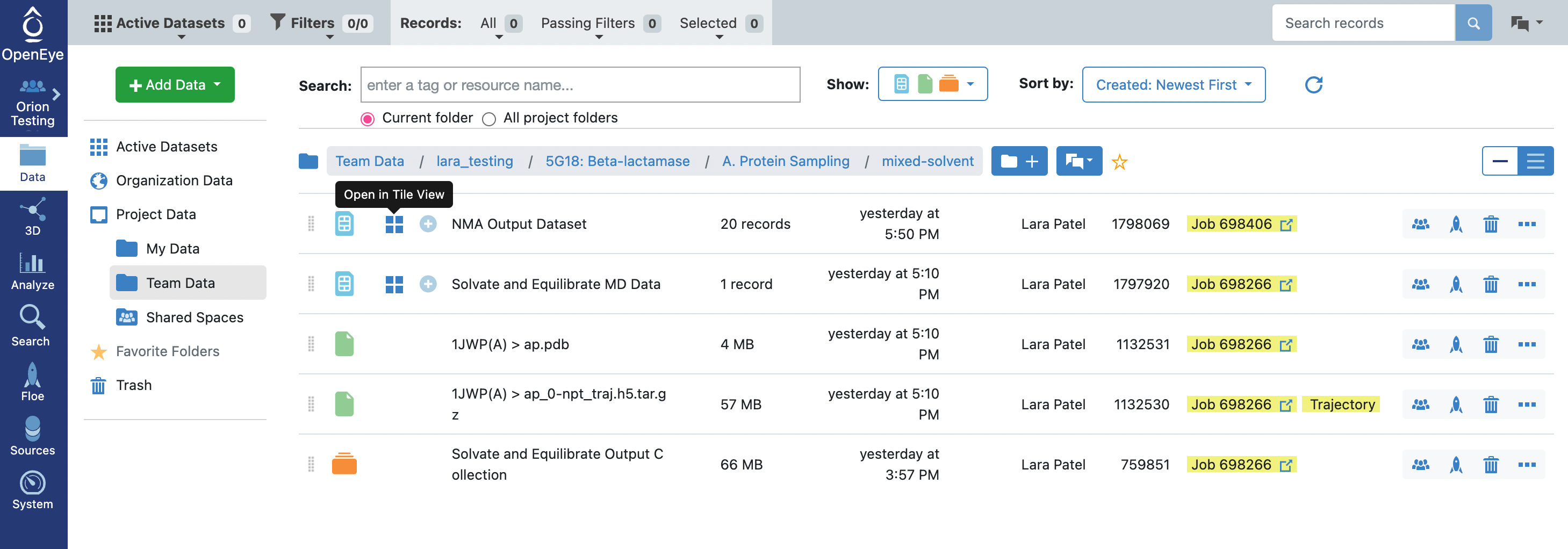
Navigate to the output dataset from the A2. Protein Sampling (for Cryptic Pockets): Calculate Normal Modes job. Open Tile View for the dataset.

In Tile View, you will unfortunately be unable to view the protein with the depiction of the orange arrows representative of the mode vectors. However, you will be able to see the Mode Index and Mode Collectivity by clicking on the Columns icon and toggling those record fields to be visible.

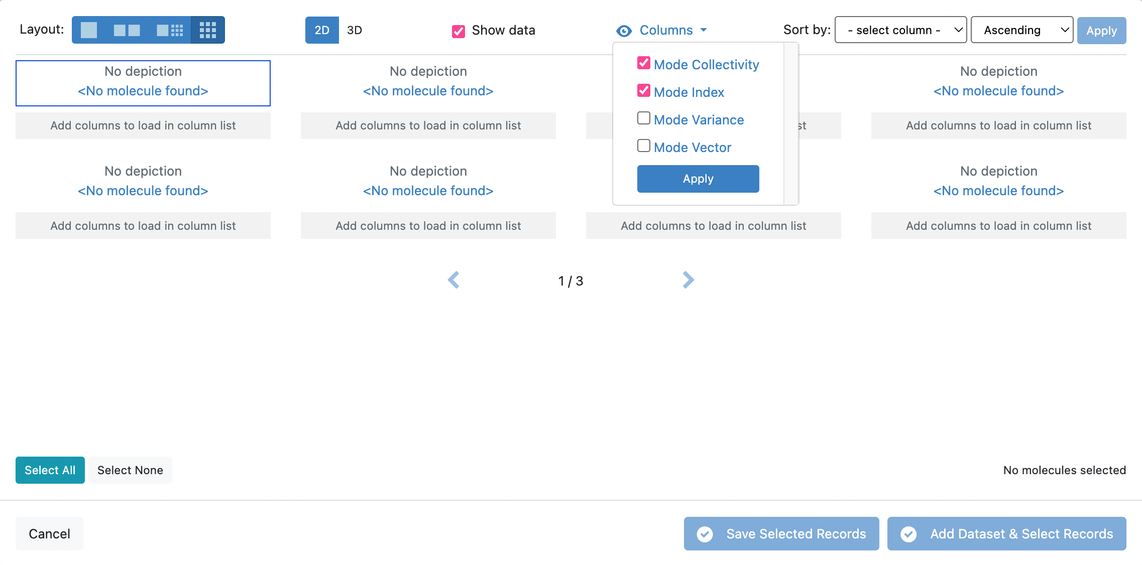
Now sort the records by the Mode Collectivity by changing the Sort by: fields to match what is depicted in the snapshot below in Descending order.

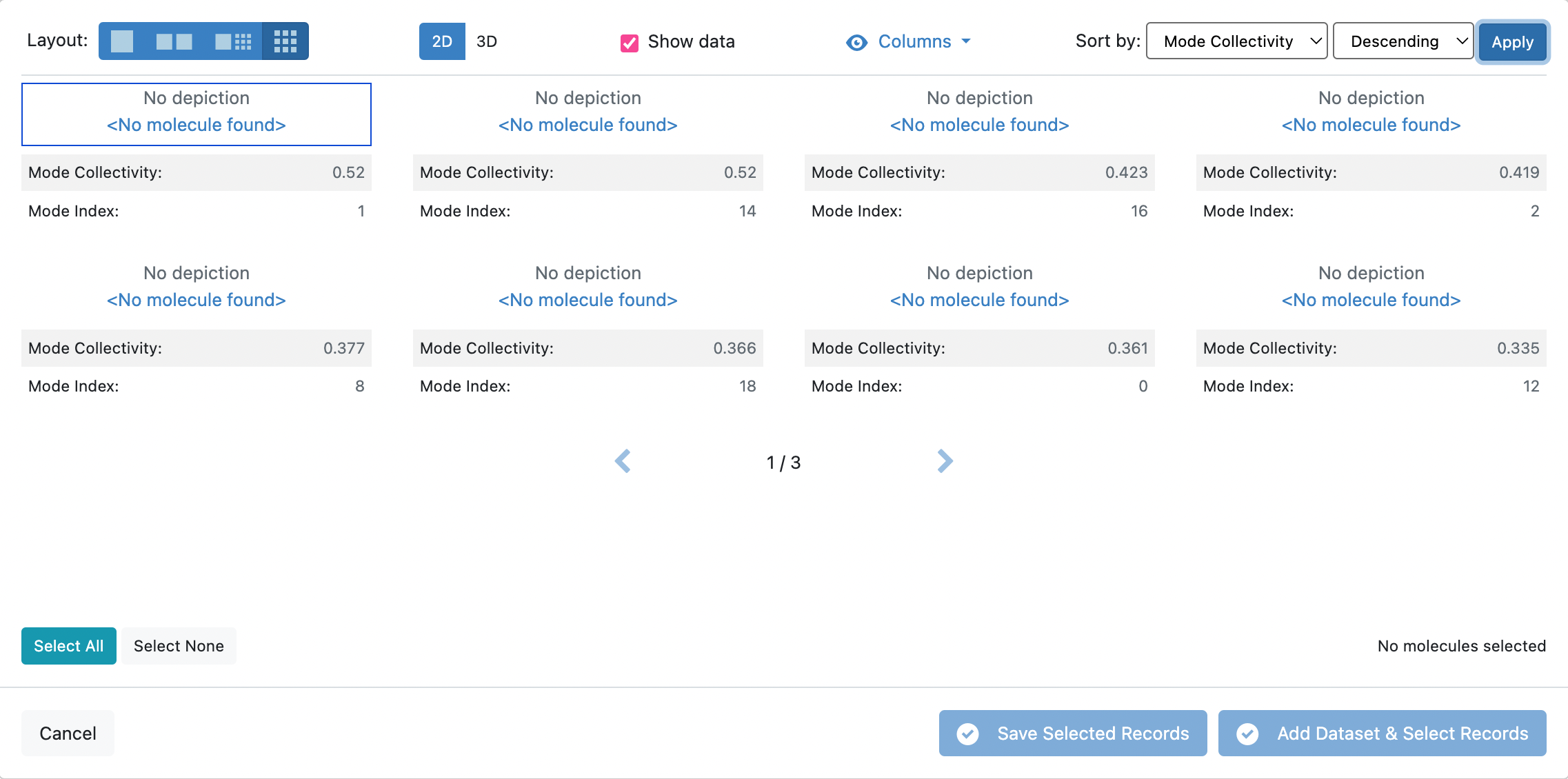
In this tutorial, we shall select the first two records with the highest Mode Collectivity.

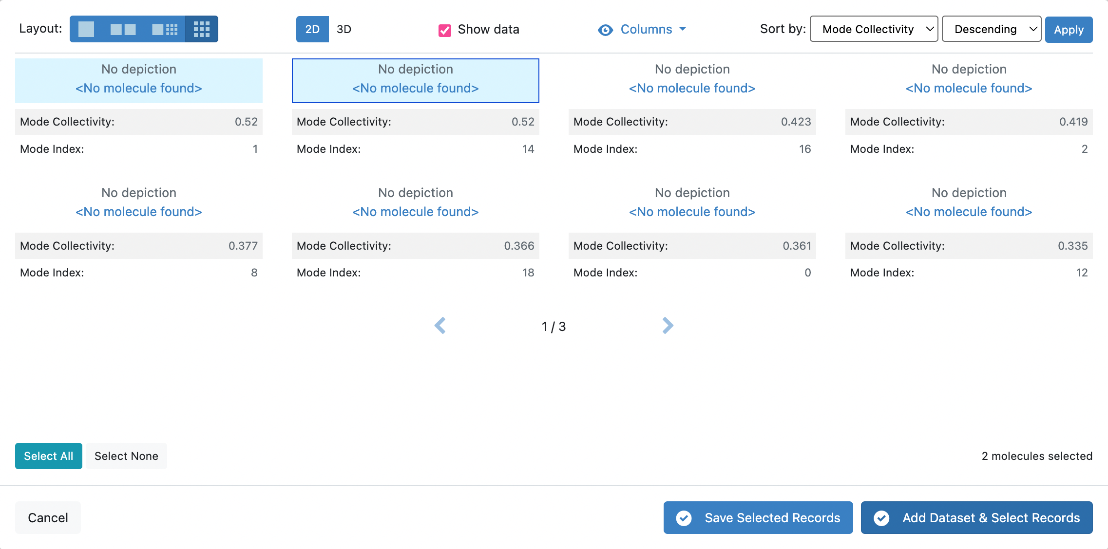
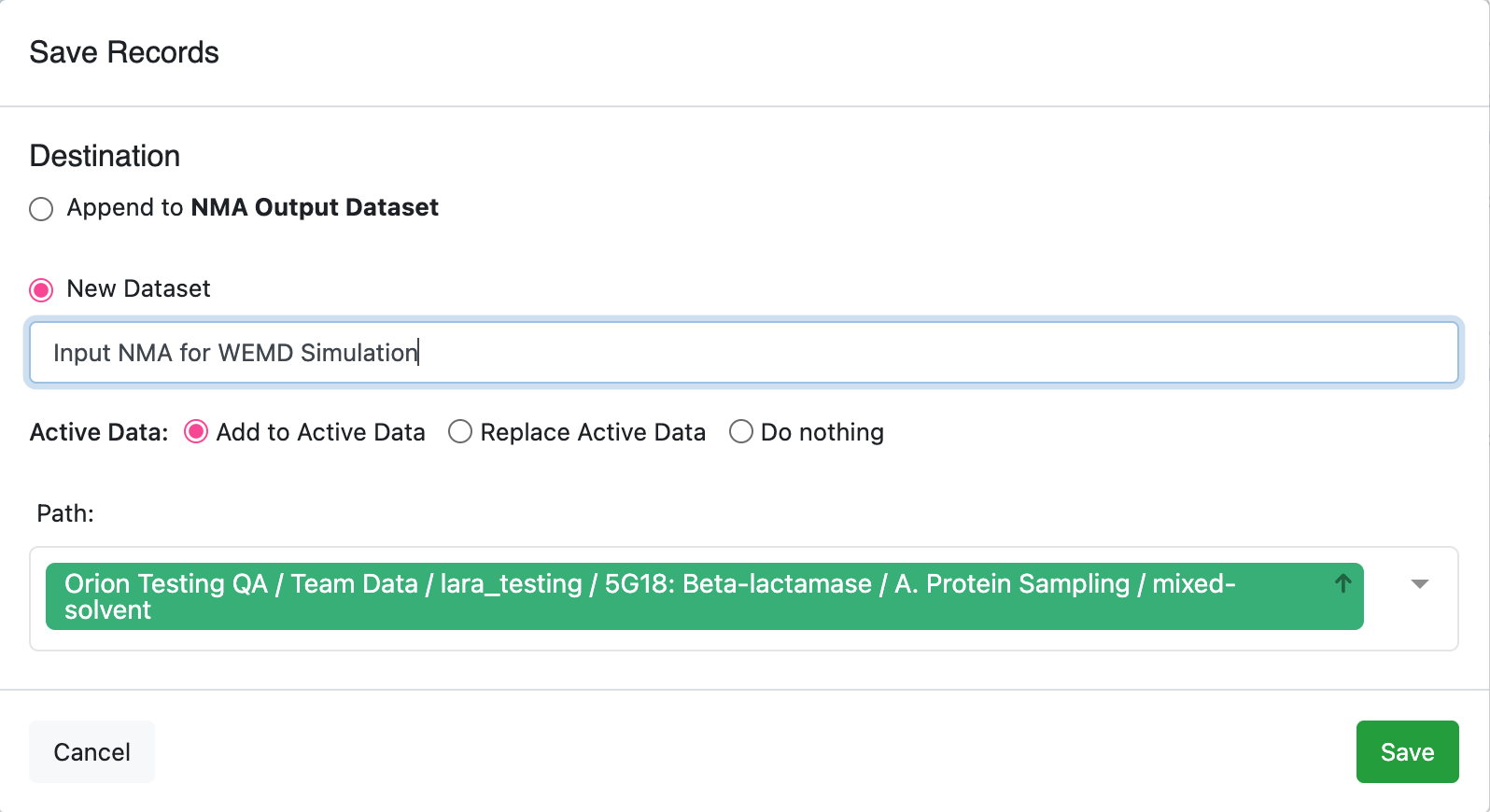
Click the blue Save Selected Records button at the bottom of the page. Give the dataset a name that you will remember. This dataset will contain only the two modes that are going to be used as input for the weighted ensemble simulation.

At this point, navigate to the blue navigation side bar Floe tab and click on the Floes tab at the top of the page. Then search for A3a. Protein Sampling (for Cryptic Pockets): Run a Weighted Ensemble MD Simulation and click on the LAUNCH FLOE button to open the floe options. Proceed to the Running the WEMD Simulation Floe instructions.

Selecting Input Normal Modes (Option 2)

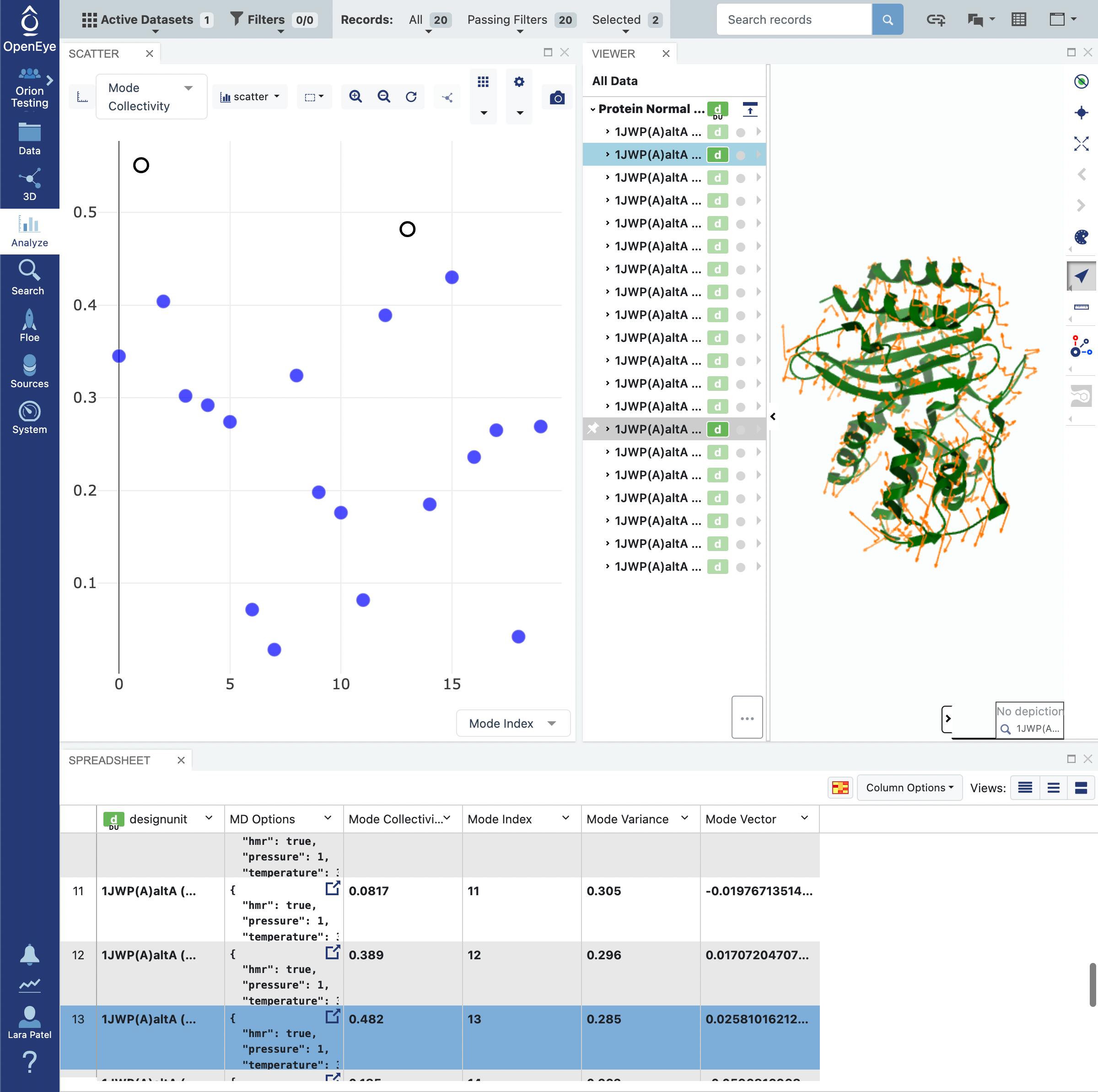
Click on the blue navigation side bar Analyze tab. Make sure that the normal mode output dataset is the Active Datasets. Make sure that your analysis page is set up to view the representative protein structure with the normal mode represented with orange arrows for the mode vectors. This is done by clicking on the Layout icon in the top right corner of the page and selecting Analyze with 3D. Make sure that the y-axis of the scatter plot shows the Mode Index and the x-axis shows the Mode Collectivity.

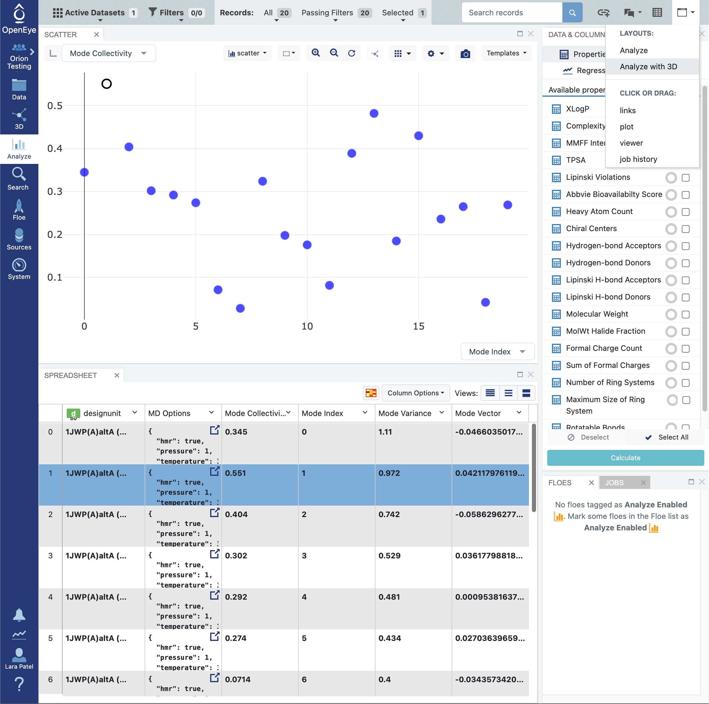
Clicking on a single data point on the scatter plot will display the representative structure and the normal mode vectors for that dataset record.

You can select multiple data points by using the click and drag selection box or by holding the command key on your keyboard and clicking on data points. Select the two highest collectivity modes.

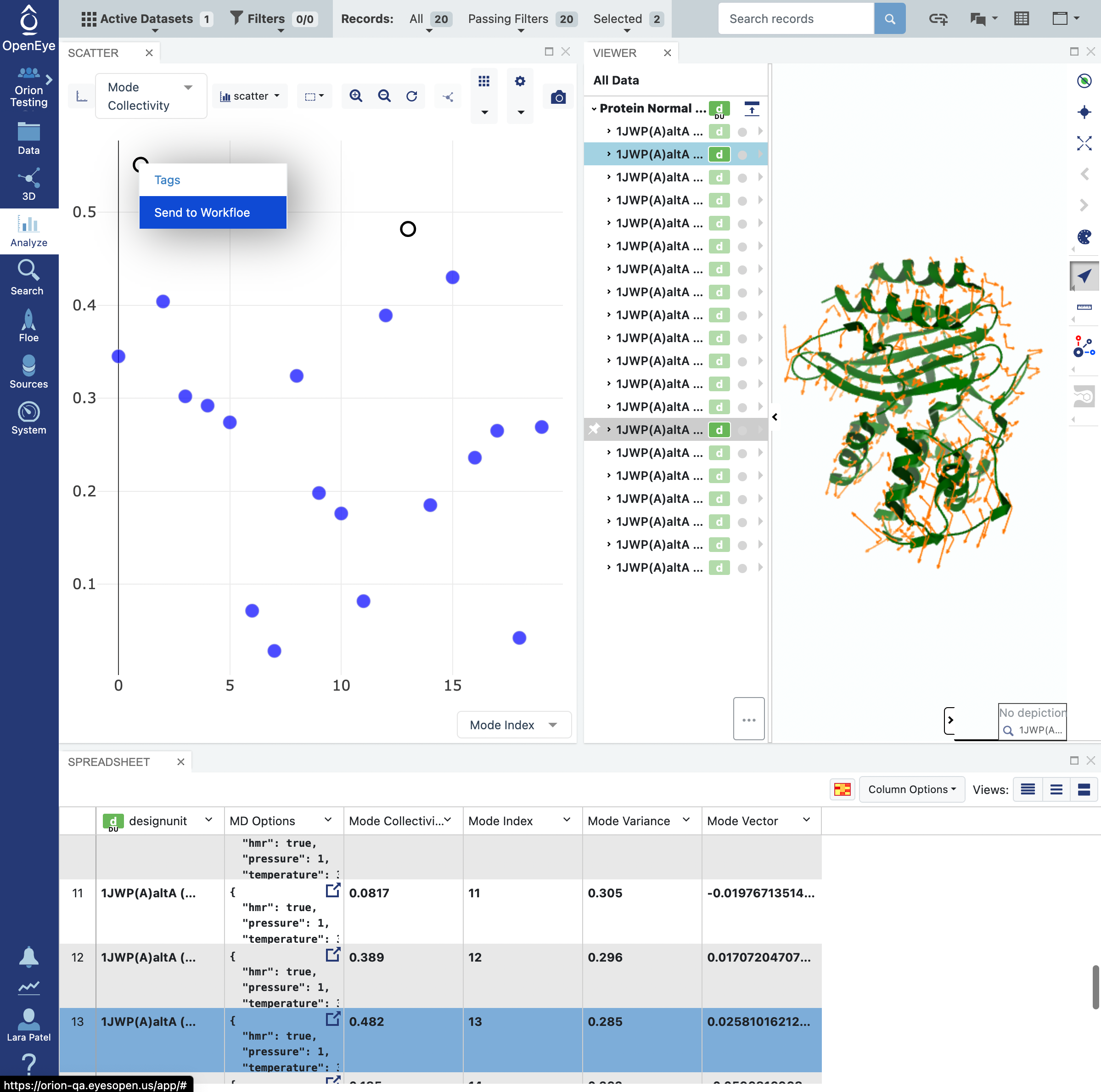
Right click on one of the selected modes to activate a drop-down menu. Select the Send to Workfloe option.

The window that opens will give you the option to select an existing workfloe or to search for the floe as seen below.

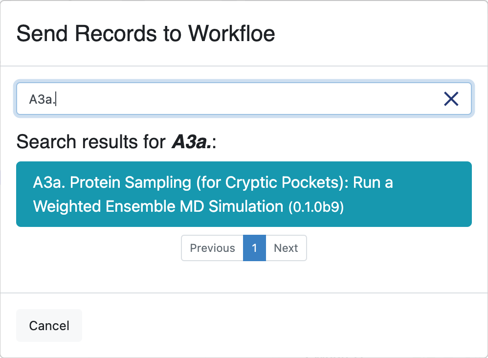
Click on the A3a. Protein Sampling (for Cryptic Pockets): Run a Weighted Ensemble MD Simulation Floe. This will redirect you to the floe options page. The selected records will auto-fill the first input dataset field of the floe options. Make sure that they have been assigned to the Inputs -> Protein Normal Mode Records field. You can change the assigned field by clicking on the inverted triangle on the Choose Input button for the correct field.

Running the WEMD Simulation Floe

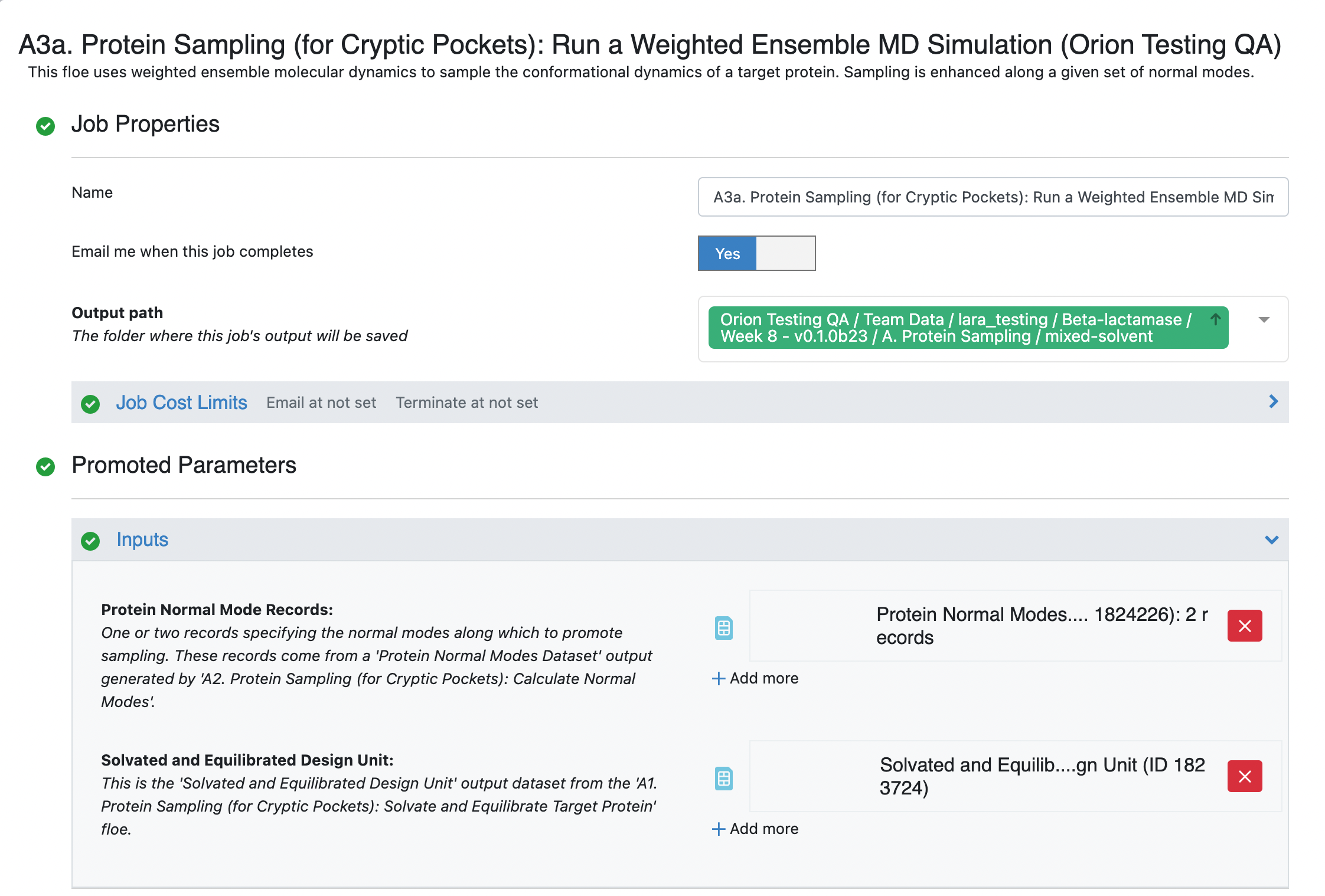
Select the desired Output Path. Fill out the following input parameters:

• Protein Normal Mode Records: If you choose Selecting Input Normal Modes (Option 2), this field should be already populated by the input records. If you choose Selecting Input Normal Modes (Option 1), add the records/dataset that you saved by selecting one or two normal mode records from the dataset generated by the A2. Protein Sampling (for Cryptic Pockets): Calculate Normal Modes.

• Solvated and Equilibrated Design Unit: Select the design unit output generated by the A1. Protein Sampling (for Cryptic Pockets): Solvate and Equilibrate Target Protein Floe. The default output dataset name is Solvated and Equilibrated Design Unit.

You can customize the file names under the Outputs options, but in this case, we have used the default values. Set the Weighted Ensemble Parameters -> Iterations field to 5 (or 48 for the long run) and set the Advanced Weighted Ensemble Parameters -> Trajectories Per Bin to 5. For a production simulation, we recommend leaving the trajectories per bin at the default value of 10, but for the sake of making the tutorials cheaper to run, a value of 5 makes more sense.

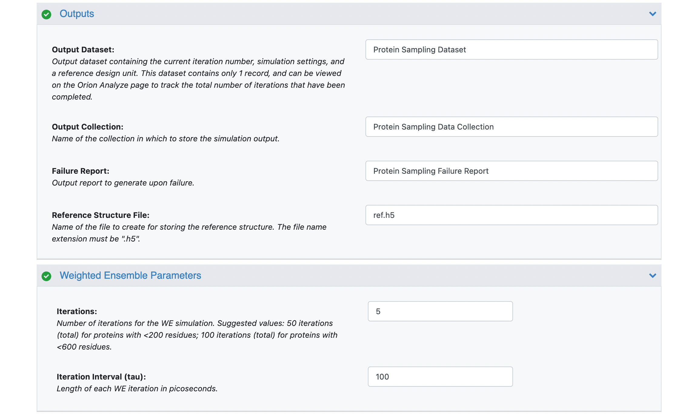
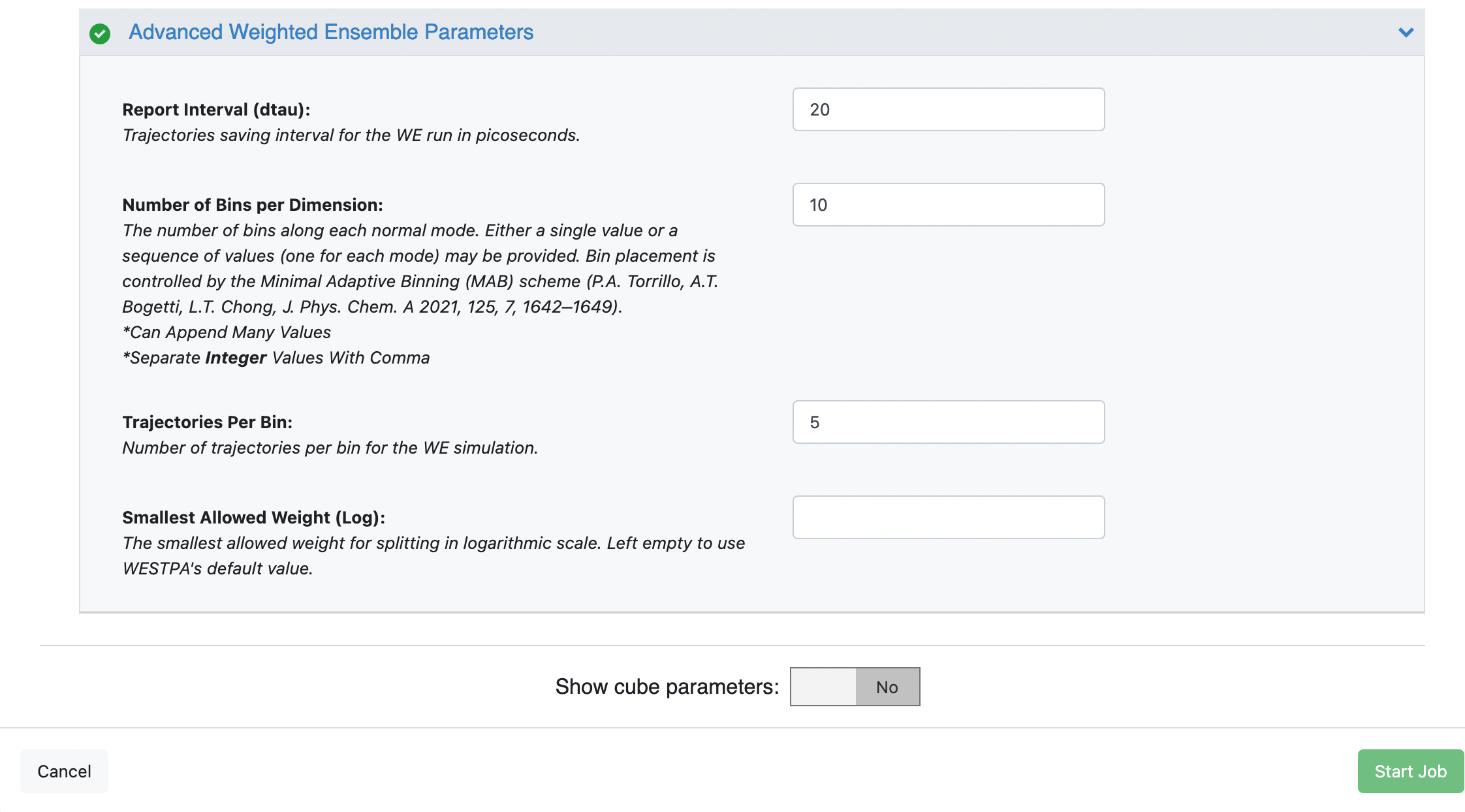
Once your floe parameters have been set, click on the Start Job button at the bottom of the window. The floe will generate three outputs: a dataset, a collection, and an h5 file.

It should be noted that you can keep track of the progress of your simulation job once the output dataset has been generated. Navigate to the data for the job by clicking on Floe tab of the vertical navigation bar, clicking on the Jobs tab of the horizontal navigation bar and then clicking on the Job itself. This will redirect you to the Floe view of the job and in the upper left corner, under Results, you should see your output dataset name and a blue link for Show in Project Data. Click on that link and then click on on the circle with a + sign in the middle next to the Protein Sampling Dataset for the job that is actively running and then viewing the dataset in the Analyze page by clicking on the Analyze tab of the vertical navigation bar.

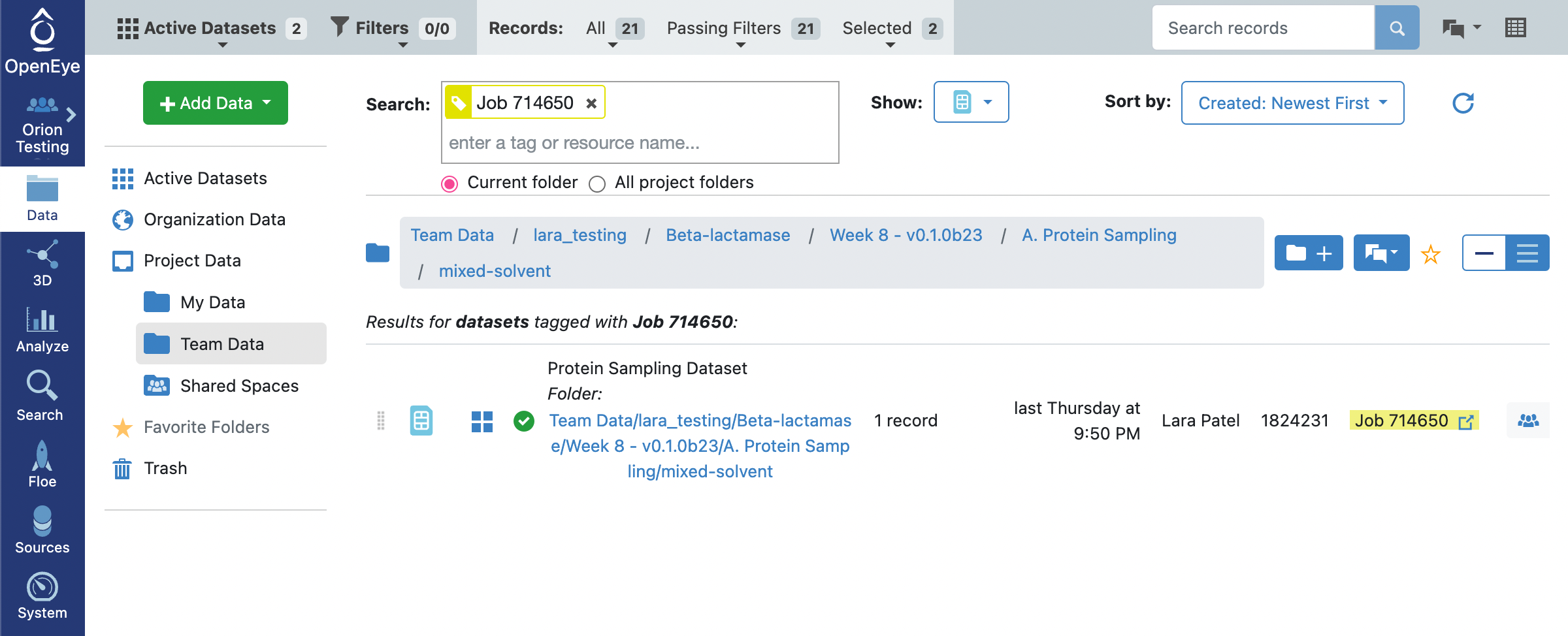
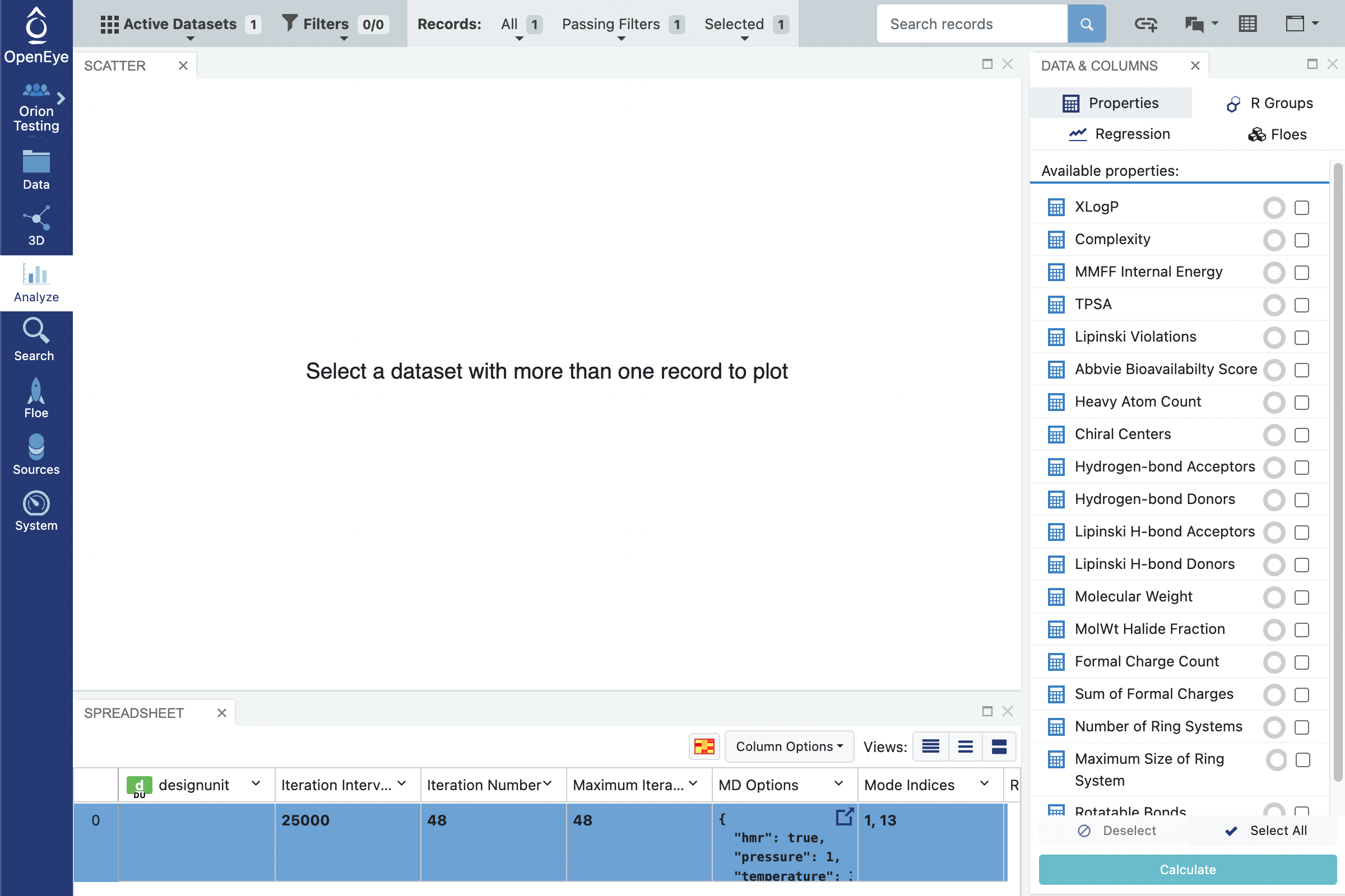
In the snapshot above you can see that the iteration number (column 3) is currently at 48 for your simulation that has reached completion but for a running simulation this number will indicate the number of completed iterations to date. The Maximum iterations field (column 4) keeps track to the total number of iterations for the simulation to complete. The mode indices field indicate the modes that were chosen as the input progress coordinates. In the snapshot above, you can see that modes 1 and 13 were chosen.

Tip

Wait for the submitted job to finish. If you are running a 5 iteration simulation, the job will complete in 1-2 hours and cost approximately $10. However, if you are running the larger simulation with 48 iterations, this will take 13-16 hours to complete and cost approximately $150. If you are running the later, this is a good time to take a break and check in the next day on the simulation to make sure it is complete before proceeding to the next step.

Tip

If your simulations get interrupted or are cancelled, the collection will be left open. In order to close it, please run the A3b. Protein Sampling (for Cryptic Pockets): Continue a Weighted Ensemble MD Simulation Floe for one or two iterations. This will facilitate closing the collection correctly.

Continue a Weighted Ensemble MD Simulation (Optional)

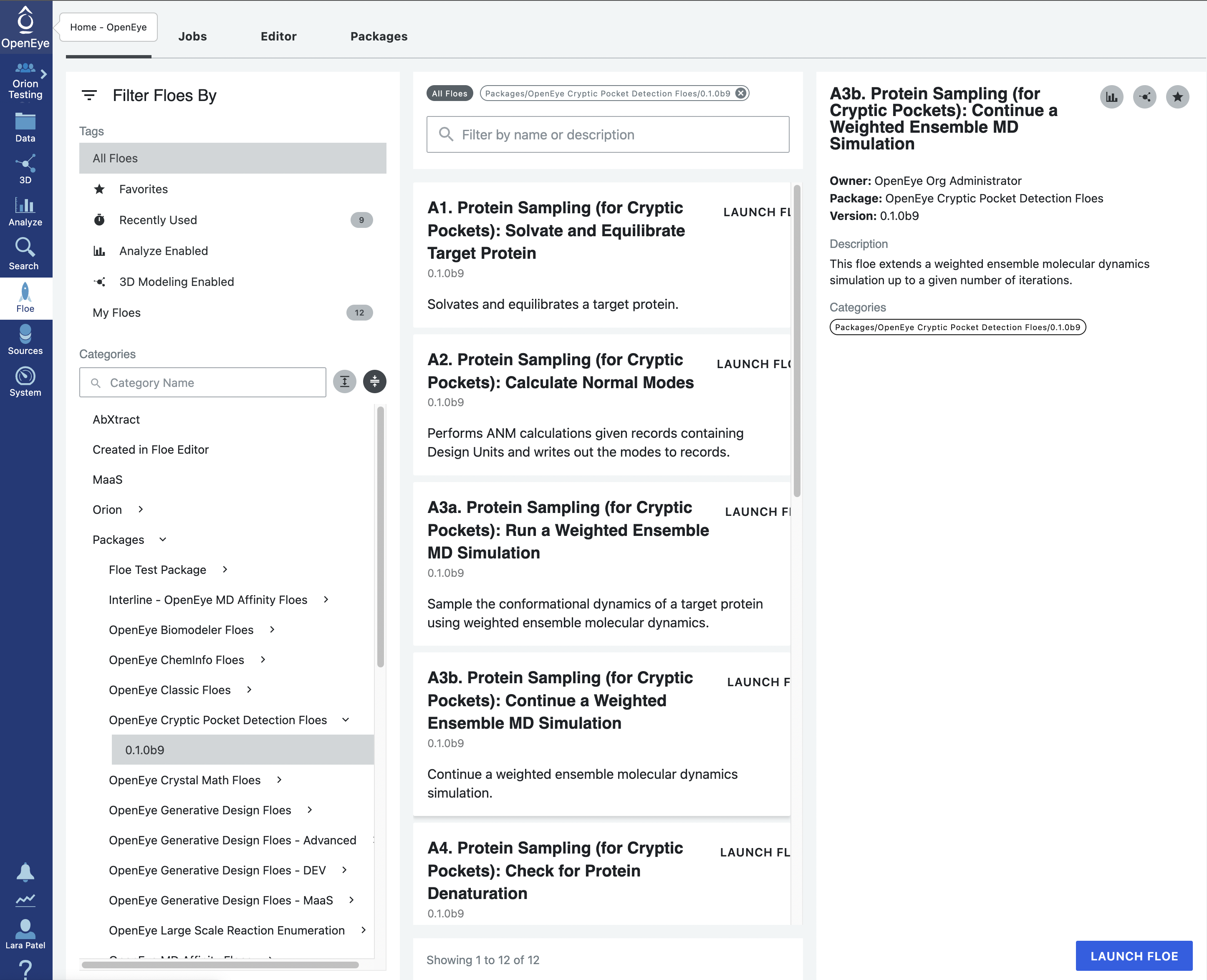
To continue the weighted ensemble simulation, click on the blue navigation side bar Floe tab and then click on the Floes tab at the top of the page. Filter the Packages -> OpenEye Cryptic Pocket Detection Floes and select the A3b. Protein Sampling (for Cryptic Pockets): Continue a Weighted Ensemble MD Simulation Floe. Click the blue LAUNCH FLOE button.

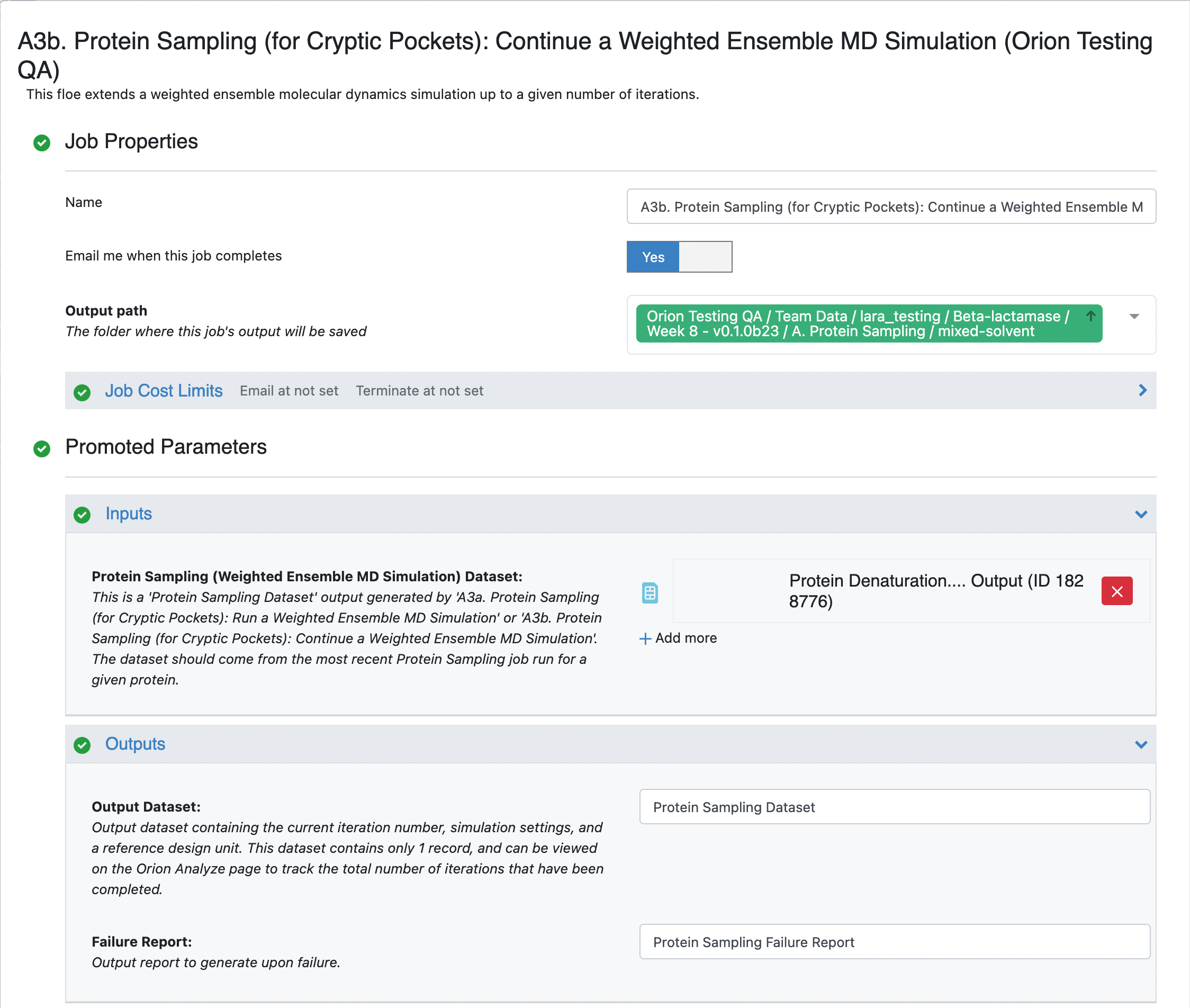
This will open the floe options page. Select the desired Output Path. Select the output dataset (which will contain a single record) from the previous floe as the Input -> Input Record to this floe. Note that this floe will append to the existing collection that was created when running the previous floe. Input a value of 5 for the Weighted Ensemble Parameters -> Additional Iterations.

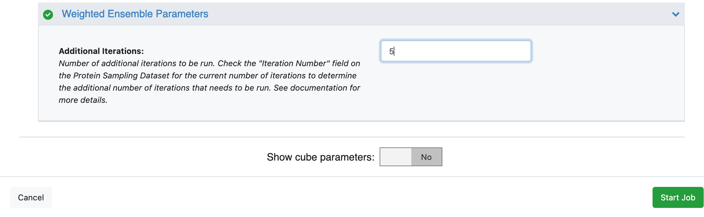
Click on the green Start Job button at the bottom of the page.

Tip

Wait for the submitted job to finish. If you are running a 5 iteration simulation, the job will complete in 1-2 hours and cost approximately $10. If you are running the additional 2 iterations on the longer simulation that previously had 48 iterations, the job should complete within an hour and cost approximately $10.

Check for Protein Denaturation (Mixed Solvent)

This floe acts as a diagnostic floe to evaluate the sampling and whether the protein is unfolding in the Weighted Ensemble MD simulations of the A3a. Protein Sampling (for Cryptic Pockets): Run a Weighted Ensemble MD Simulation and A3b. Protein Sampling (for Cryptic Pockets): Continue a Weighted Ensemble MD Simulation Floes.

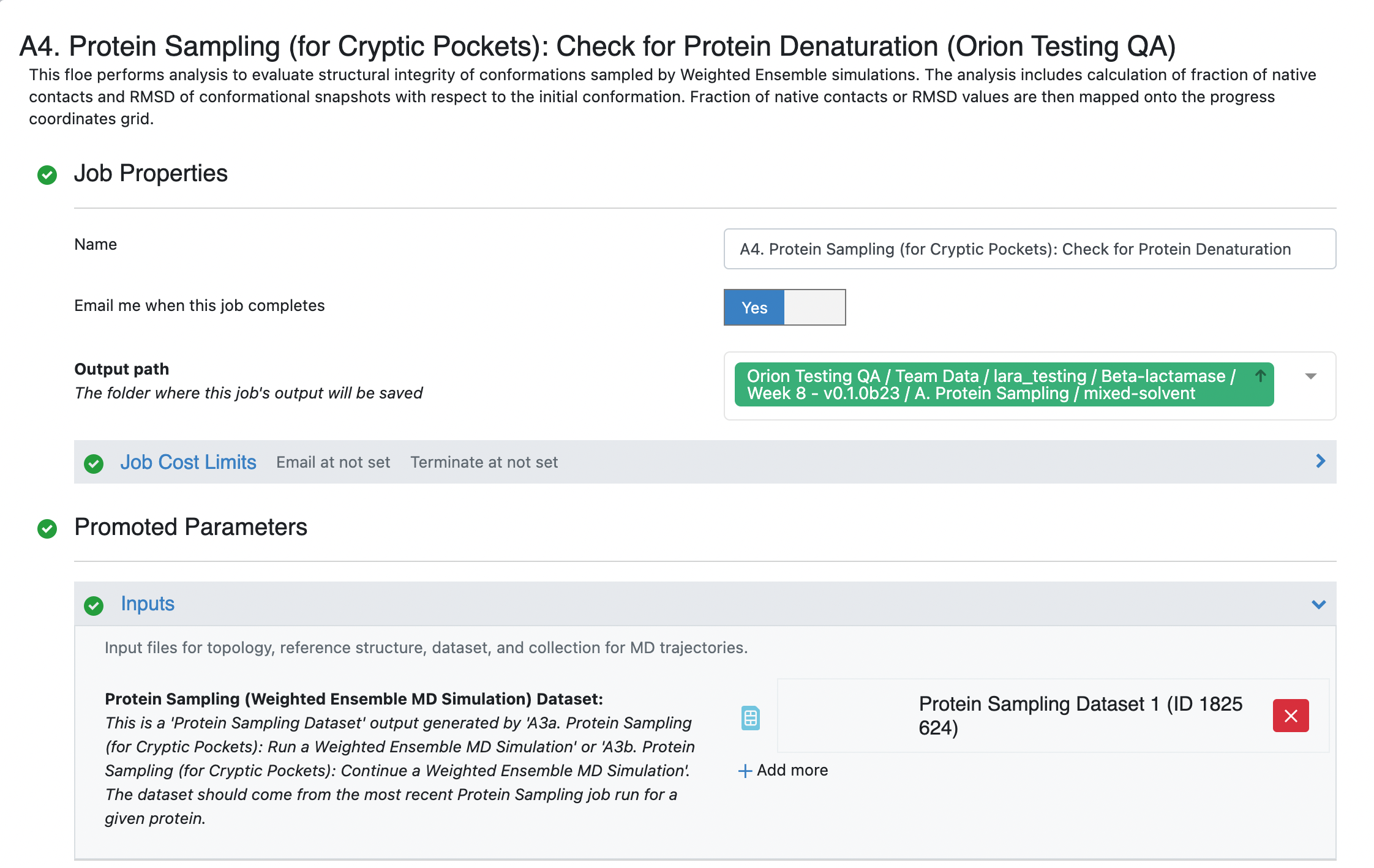
To run this floe, click on the blue Floe tab in the vertical navigation bar and the grey Floes tab in the horizontal navigation bar. There will be a light grey vertical navigation bar on the side that allows you to filter the package for which you see Floes. Click on the Packages -> OpenEye Cryptic Pocket Detection Floes option and in the search bar in the middle pane, search for the A4. Protein Sampling (for Cryptic Pockets): Check for Protein Denaturation Floe either manually by scrolling or by typing the start of the floe name into the search bar. Click on the blue LAUNCH FLOE button at the bottom of the page.

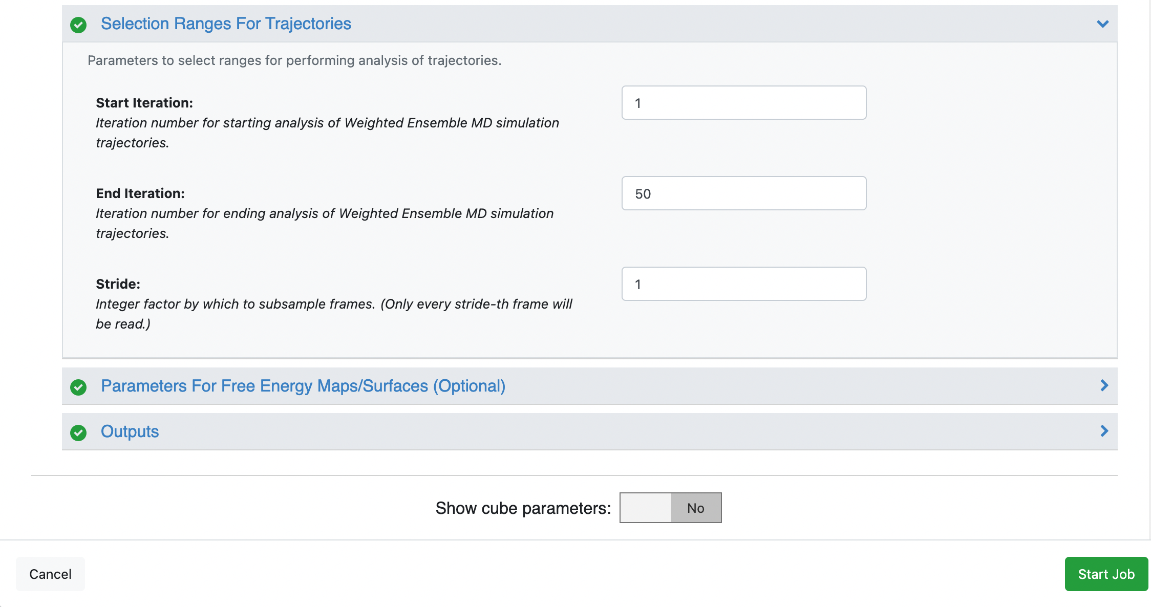
Fill out the Job parameters page by adding the last protein sampling dataset as the input dataset. Ideally this should be the dataset from the full 50 iteration simulation. If the A3b Floe was completed the output dataset name was not customized, it will probably be called Protein Sampling Dataset 1. Optionally, you can specify the End Iteration as 50. The default behavior when this field is left blank is to analyze all of the iterations leading up to the iteration of the input dataset.

Tip

Wait for the submitted job to finish. This job should take approximately 1 hour to complete and cost $15.

Once this job has completed, you will want to take a look at the Floe Report. You can either navigate to where the Floe Report collection is located in your data or you can access it through the job information. Start by clicking on the blue Floe tab in the vertical navigation bar and the grey Jobs tab in the horizontal navigation bar. Then click on the job for running this floe.

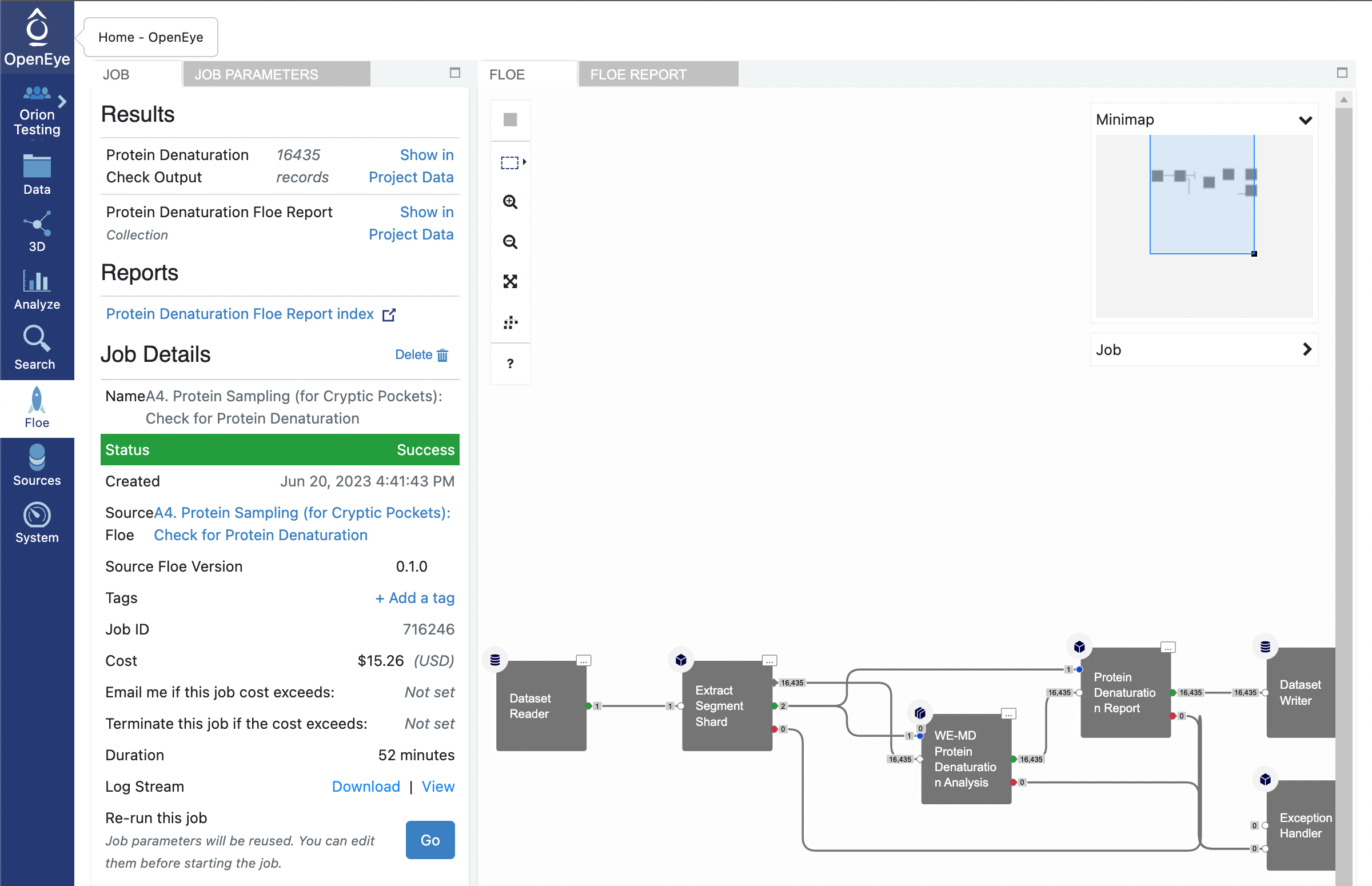
There are two columns on the Job summary page. The left most column has two tabs JOB and JOB PARAMETERS, and the right most column has two tabs FLOE and FLOE REPORT. Click on the FLOE REPORT tab. The floe report may take a moment to load but you will be able to see the results. If you would like to view the floe report on a full webpage, click on the Open in a new tab button that has a square with an arrow pointing diagonally out of the upper right corner.

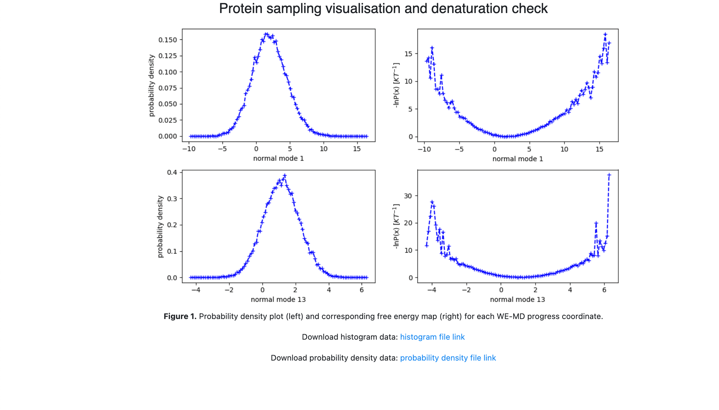
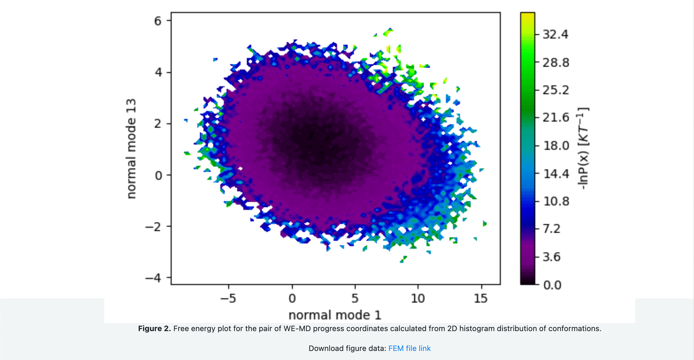
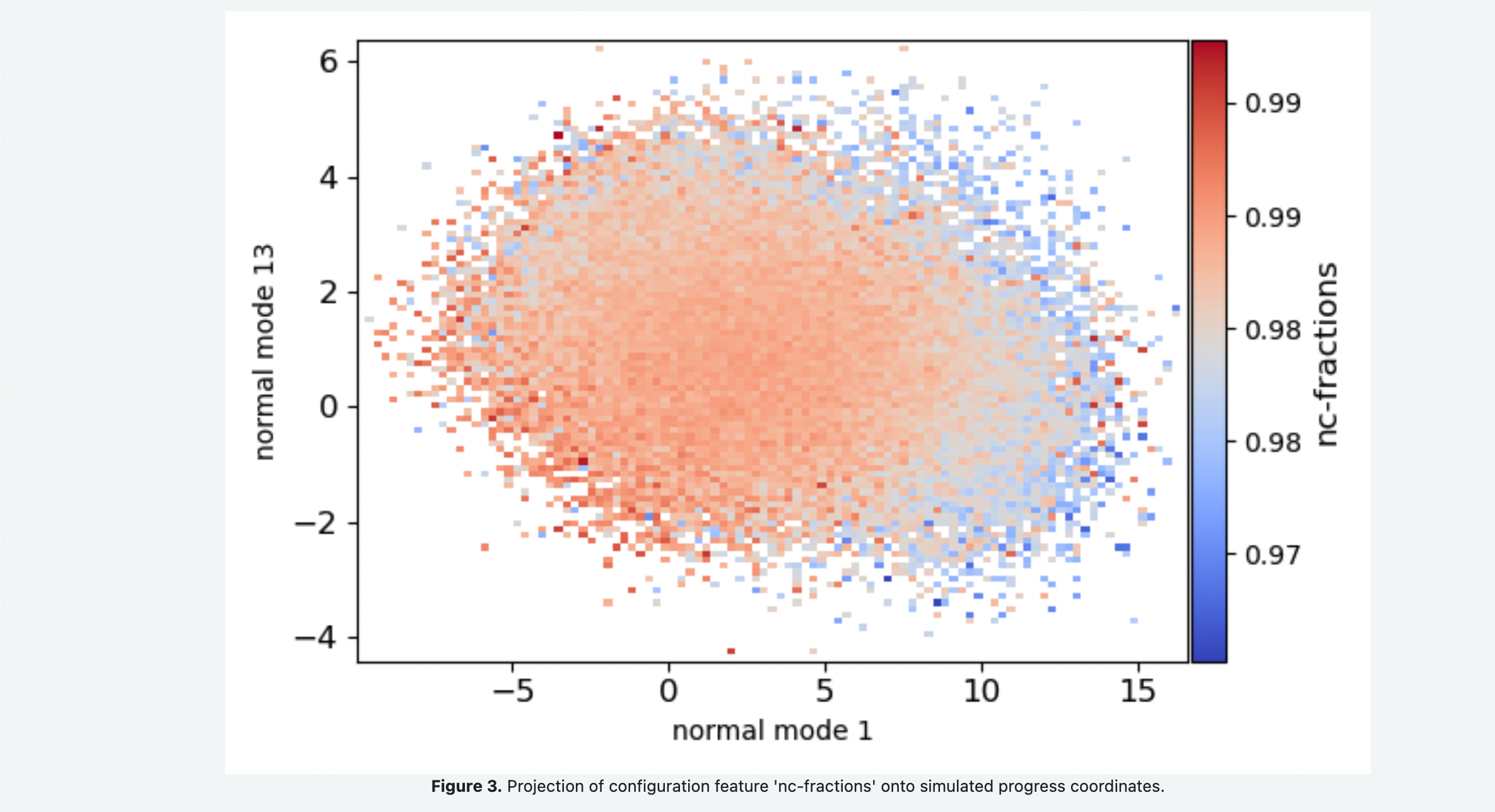
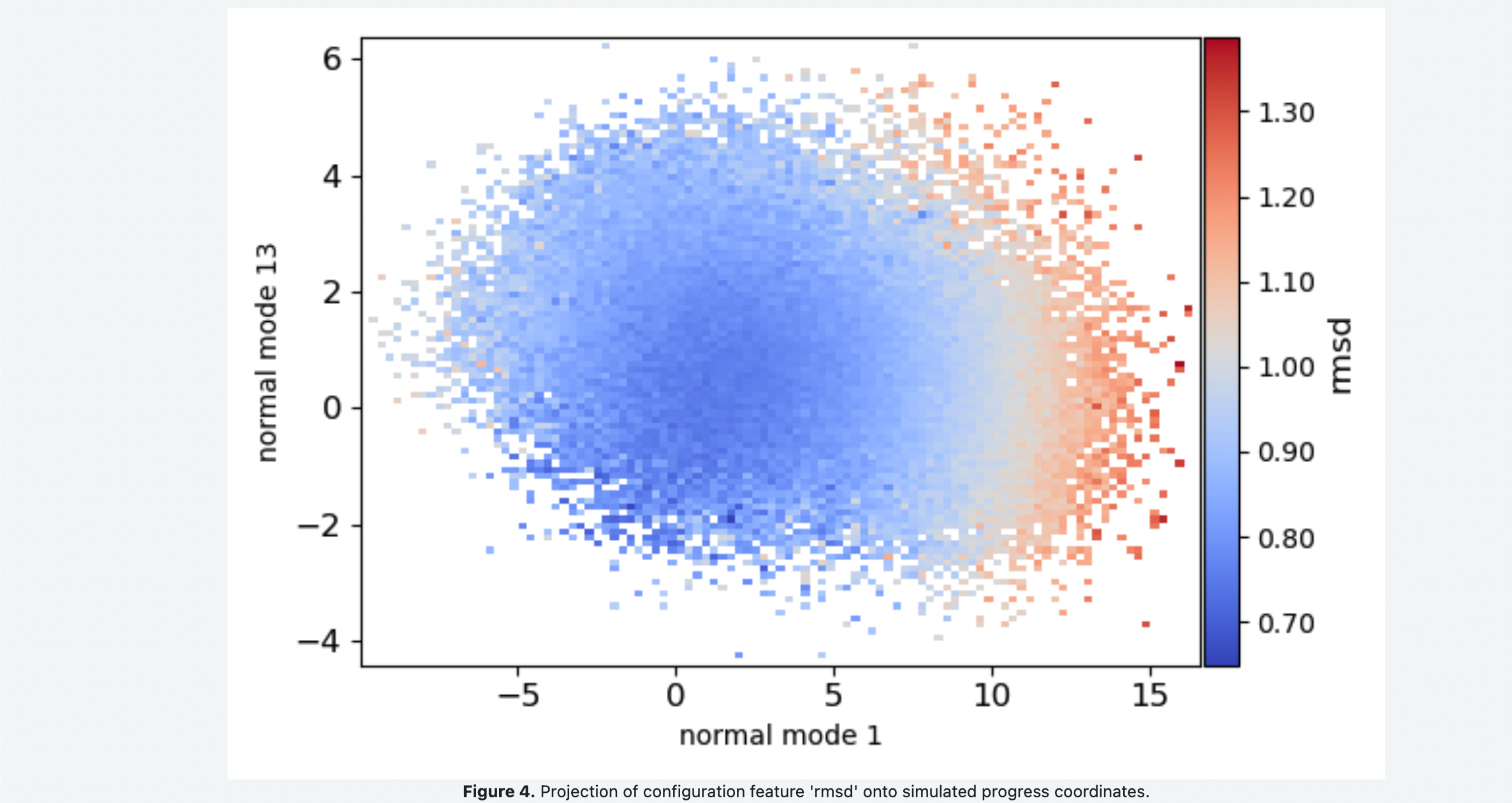
You Floe Report should look something like the following snapshots. Figure 1 shows the 1-D probability distributions and negative log of the probability distribution for each of the progress coordinate normal modes. Comparing the free energy landscape in Figure 2 as you increase the number of iterations can be used as a qualitative assessment of how well sampled and converged the simulations are. Figure 3 shows the average fraction of native contacts conserved in the simulation projected onto the progress coordinates. This can be used to assess if the protein is unfolding along the progress coordinates. Figure 4 shows the average RMSD of the conformations projected onto the progress coordinates.

Trajectory Analysis (for Cryptic Pockets)

Residue-Cosolvent Minimum Distances

This floe can only be run with the output from a mixed-solvent simulation.

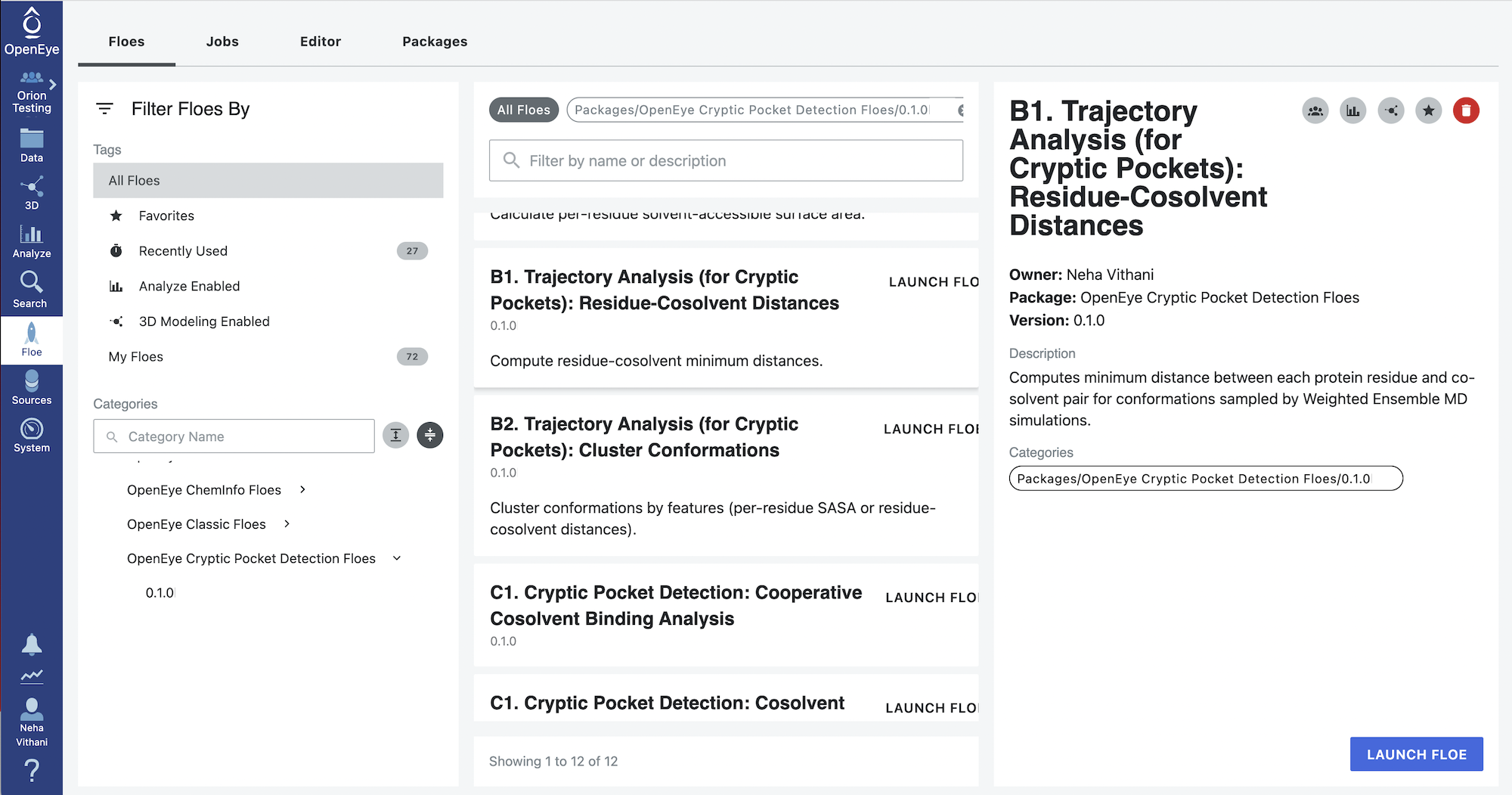
Start by clicking on the blue navigation side bar Floe tab. Click on the Floes tab at the top of the page and then filter for Packages -> OpenEye Cryptic Pocket Detection Floes. Select the B1. Trajectory Analysis (for Cryptic Pockets): Residue-Cosolvent Distances Floe and click the LAUNCH FLOE button.

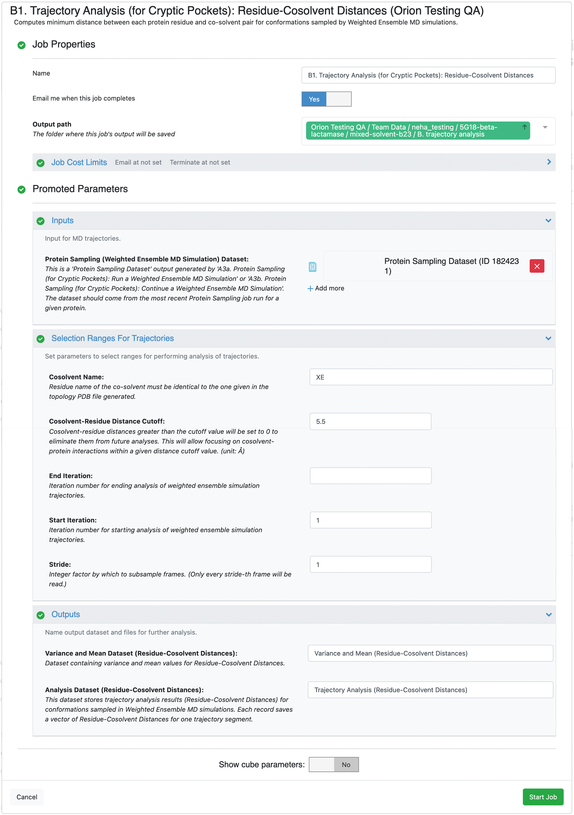
Select the desired Output Path. Fill out the following input parameters:

• Protein Sampling (Weighted Ensemble MD Simulation) Dataset: Select the most recent dataset generated by the A3a. Protein Sampling (for Cryptic Pockets): Run a Weighted Ensemble MD Simulation Floe or the A3b. Protein Sampling (for Cryptic Pockets): Continue a Weighted Ensemble MD Simulation Floe. If you did not change the output dataset name, it will be Protein Sampling Output or Protein Sampling Output 1. Orion appends integers to duplicate file names.

• Selection Ranges for Trajectories -> End Iteration: Input the iteration number (50). If it is left unspecified, the entire simulation dataset is analyzed. This parameter and the Selection Ranges for Trajectories -> Start Iteration selects the range of iterations to perform analysis on from the weighted ensemble simulations. We do not recommend excluding initial iterations from the analysis.

Note

For large simulation datasets (>100 iterations) and proteins consisting of >200 residues, we recommend analyzing the weighted ensemble simulation collection in multiple batches of approximately 50 iterations using the Selection Ranges for Trajectories -> Start Iteration and Selection Ranges for Trajectories -> End Iteration parameters.

Click on the green Start Job button at the bottom of the page.

Tip

Wait for the submitted job to finish. This floe will take up to 2.5 hours to run and cost $6 for a protein with approximately 260 residues simulated for ~50 iterations.

Cluster Conformations

This floe will cluster conformations based on the observables calculated in the B1. Trajectory Analysis (for Cryptic Pockets): Residue-Cosolvent Distances Floe.

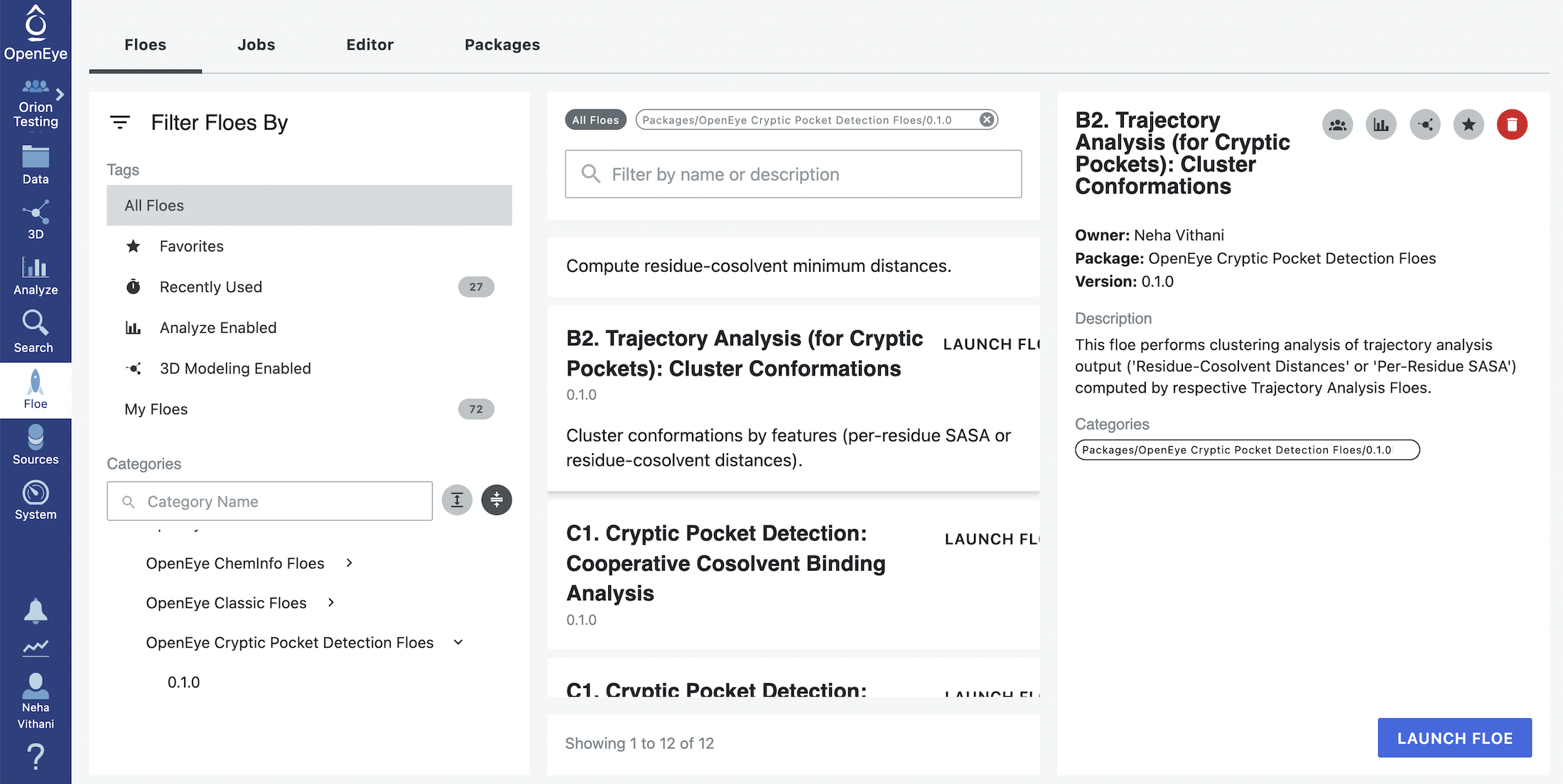
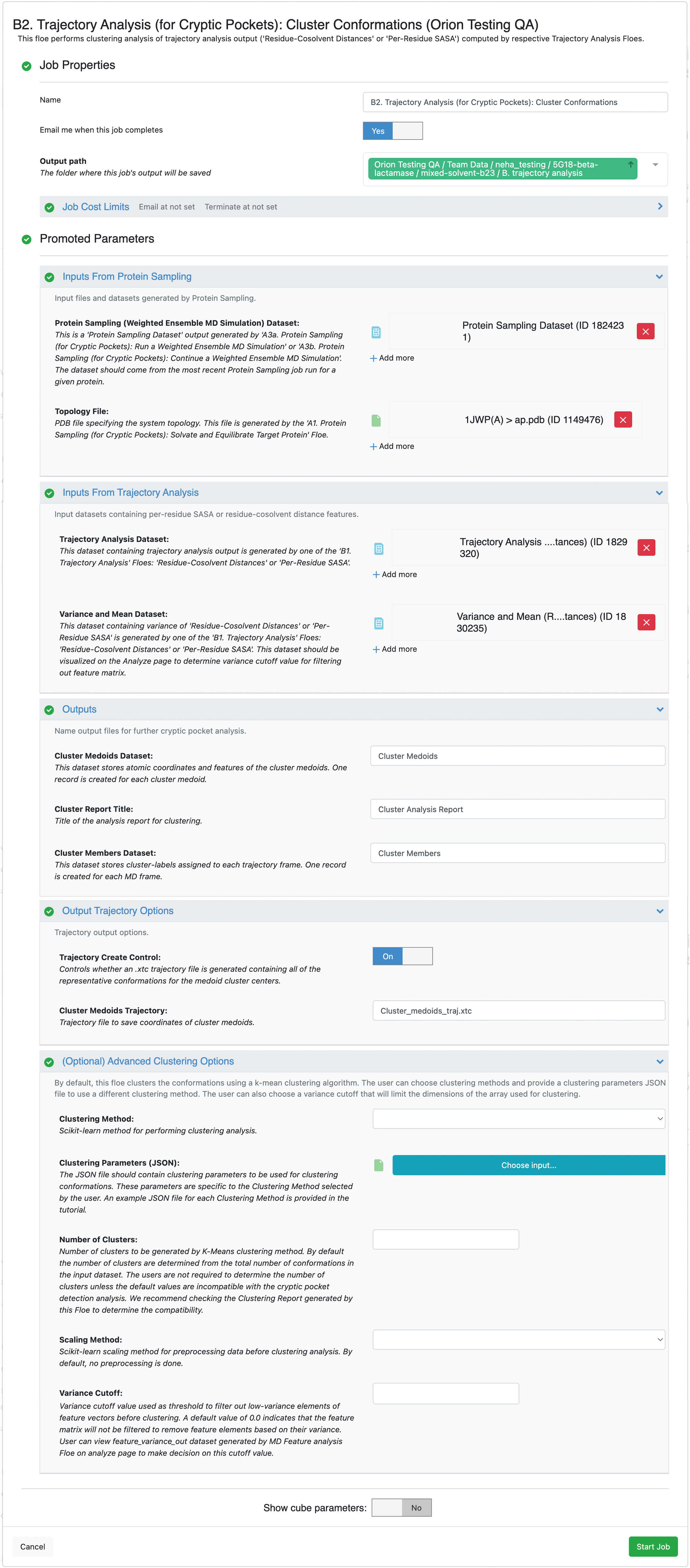
Start by clicking on the blue navigation side bar Floe tab. Click on the Floes tab at the top of the page and then filter for Packages -> OpenEye Cryptic Pocket Detection Floes. Select the B2. Trajectory Analysis (for Cryptic Pockets): Cluster Conformations and click the LAUNCH FLOE button.

Select the desired Output Path. At this stage of the analysis, you will use the output from several Floes that were run earlier in this tutorial as input for this Floe. Input files for the Inputs From Protein Sampling parameter group were generated when running the Protein Sampling (for Cryptic Pockets) Floes:

• Protein Sampling (Weighted Ensemble MD Simulation) Dataset: Select the most recent dataset generated by the A3a. Protein Sampling (for Cryptic Pockets): Run a Weighted Ensemble MD Simulation Floe or the A3b. Protein Sampling (for Cryptic Pockets): Continue a Weighted Ensemble MD Simulation Floe. If you did not change the output dataset name, it will be Protein Sampling Output or Protein Sampling Output 1. Orion appends integers to duplicate file names.

• Topology File: Select the PDB file generated by the A1. Protein Sampling (for Cryptic Pockets): Solvate and Equilibrate Target Protein Floe.

Input files specified under Select Inputs From Trajectory Analysis were generated by the B1. Trajectory Analysis (for Cryptic Pockets): Residue-Cosolvent Distances Floe:

• Trajectory Analysis Dataset: Provide one or more Trajectory Analysis (Residue-Cosolvent Minimum Distances) datasets generated by the B1. Trajectory Analysis (for Cryptic Pockets): Residue-Cosolvent Distances Floe.

• Variance and Mean Dataset: Provide one Variance and Mean (Residue-Cosolvent Minimum Distances) dataset corresponding to the Trajectory Analysis Dataset input selected above.

Warning

If you broke the simulation analysis in the B1 Floe into batches, provide all of the batched analysis outputs as Trajectory Analysis Dataset inputs. This analysis is intended to be run on all of the iterations leading up to the chosen maximum iteration. In contrast, you will provide only one of the Variance and Mean Datasets. We recommend using the dataset from the end batch. The weighted ensemble simulations later iterations are likely to have more bins populated with trajectory walkers.

Since the clustering Floe and its outputs are agnostic to the type of dataset being analyzed, we recommend adding (Residue-Cosolvent Minimum Distances) as a suffix to the default names given for the outputs: Cluster Medoids Dataset, Cluster Report Title, and Cluster Members Dataset.

(Optional) Advanced Clustering Options are not required as inputs unless it is recommended in the Cluster Analysis Report generated by this job.

Click on the green Start Job button at the bottom of the page.

Tip

Wait for the submitted job to finish. This Floe will take up to 9 hours to run and cost $27 for a protein with approximately 260 residues simulated for ~50 iterations.

Warning

The amount of time that the B2 floe takes greatly varies for a given simulation dataset depending on whether you are analyzing the output from the B1. Trajectory Analysis (for Cryptic Pockets): Per-Residue SASA Floe or the B1. Trajectory Analysis (for Cryptic Pockets): Residue-Cosolvent Distances Floe. The reason it takes a different amount of time is the size of the feature vectors being clustered is different. In the case of the Per-Residue SASA analysis, the feature vectors have a size less than or equal to the number of residues. The Residue-Cosolvent Minimum Distances analysis’ feature vector has a size less than or equal to the number of residues times the number of cosolvent residues. This much larger feature vector means that the clustering is more demanding and will take longer to complete.

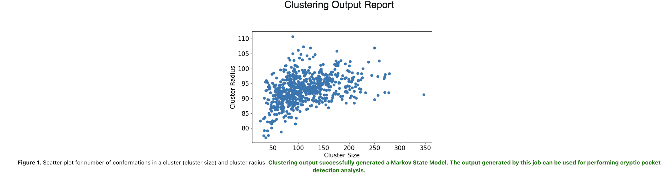
This Floe clusters the input data and then evaluates the compatibility of the clustering output for the subsequent cryptic pocket detection analysis. The Cluster Analysis Report displays the following messages depending on the suitability of the outcome for running the C1. Cryptic Pocket Detection: Cooperative Cosolvent Binding Analysis and C1. Cryptic Pocket Detection: Cosolvent Binding Free Energy Analysis Floes in the next step:

• Suitable (in green-colored text): Clustering output successfully generated a Markov State Model. The output generated by this job can be used for performing cryptic pocket detection analysis.

• Unsuitable (in red-colored text): Clustering output is not compatible with the Markov State Model estimation, and the output generated by this job can not be used for cryptic pocket detection. The Clustering Floe should be re-run by using a smaller number of cluster centers. This can be done by setting the value of ‘Number of Clusters’ input parameter to a number smaller than xxx (total number of clusters generated in this job). More details on choosing this parameter can be found in the tutorial.

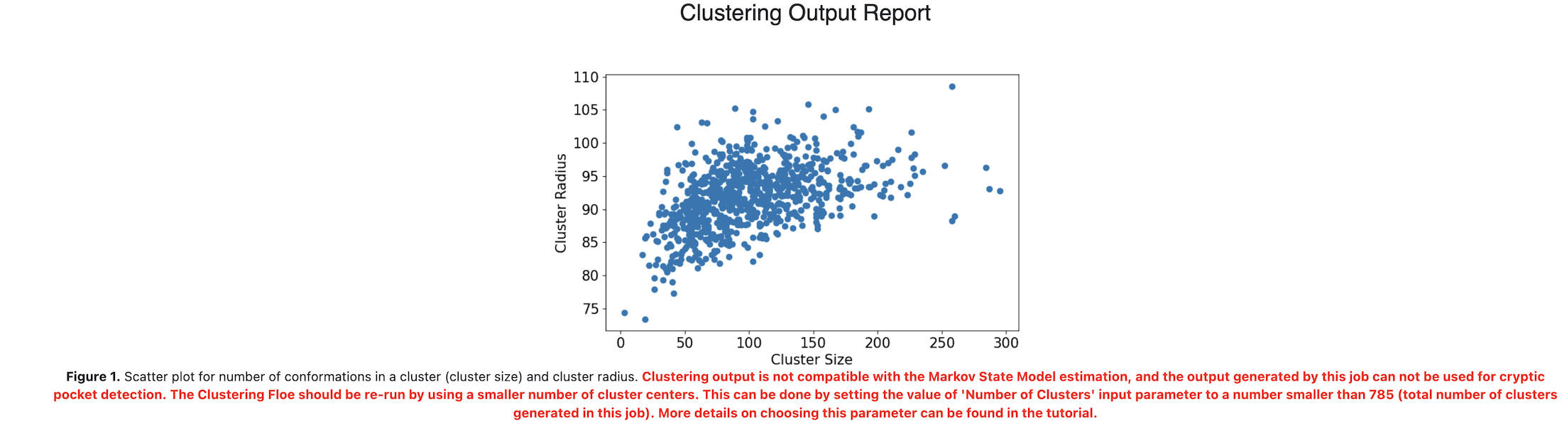
If the second message (unsuitable outcome) appears in the Cluster Analysis Report, input a number smaller than the total number of clusters generated in this job into the Number of Clusters under (Optional) Advanced Clustering Options, and re-run the Floe.

Cryptic Pocket Detection

Cosolvent Binding Free Energy Analysis

This floe can only be run with the output from a mixed-solvent simulation. This method detects pockets by finding sites with low binding free energy for the co-solvent molecules.

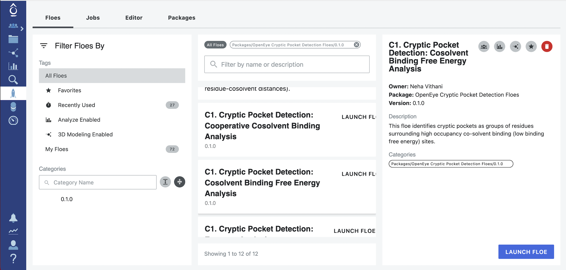
Start by clicking on the blue navigation side bar Floe tab. Click on the Floes tab at the top of the page and then filter for Packages -> OpenEye Cryptic Pocket Detection Floes. Select the C1. Cryptic Pocket Detection: Cosolvent Binding Free Energy Analysis Floe and click the LAUNCH FLOE button.

Warning

There are three distinct floes indexed as C1. Be careful to select the one whose full title is C1. Cryptic Pocket Detection: Cosolvent Binding Free Energy Analysis for the current analysis.

Select the desired Output Path.

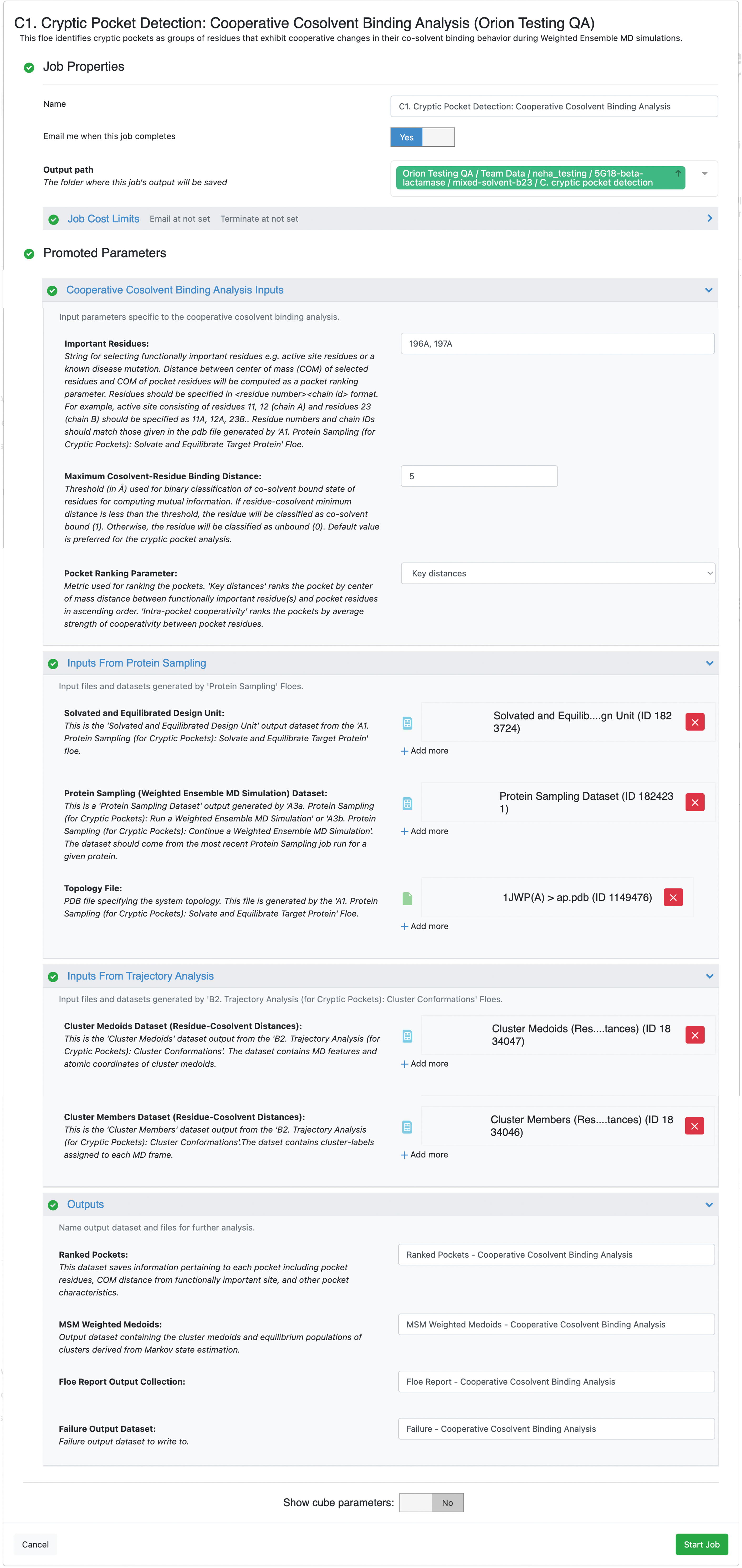
Define input parameters under the Cosolvent Binding Free Energy Analysis Inputs section:

• Medoids Trajectory File: Input the trajectory file generated by the B2. Trajectory Analysis (for Cryptic Pockets): Cluster Conformations Floe. This file is likely to be named Cluster_medoids_traj.xtc if you used the default output file name or Cluster_medoids_traj (Residue-Cosolvent Distances).xtc if you renamed the file to indicate the B1 Floe variant that generated it.

• Important Residues: In this tutorial, enter 196A,197A as the input. These residues belong to a known allosteric ligand binding site in beta-lactamase.

  The input for this parameter should be specified as a list of <residue number><chain id> formatted strings. Distance between the center of mass (COM) of these user-selected residues and the COM of pocket residues will be computed for ranking the pockets if the Key distances option is selected for the Pocket Ranking Parameter. These residues could be either functionally important residue(s) (e.g., an active site) or a known disease mutation. The residue numbers and chain IDs provided should match those given in the PDB file generated by the A1. Protein Sampling (for Cryptic Pockets): Solvate and Equilibrate Target Protein Floe. We recommend downloading the PDB file and opening it in the software of your choice to determine the residue numbers and chain IDs since the A1 Floe renumbers residues to start at 1.

• Pocket Ranking Parameter: In this tutorial, you will select the Key distances.

  By default, the Key distances option is used for ranking the pockets by their distance from the user-selected Important Residues. Cosolvent binding free energy ranks the pockets by average cosolvent binding free energy at the pocket site.

Input files required for the Inputs From Protein Sampling are those generated by running the Protein Sampling (for Cryptic Pockets) Floes in the previous steps.

• Solvated and Equilibrated Design Unit: Select the design unit output generated by the A1. Protein Sampling (for Cryptic Pockets): Solvate and Equilibrate Target Protein Floe. The default output dataset name is Solvated and Equilibrated Design Unit.

• Protein Sampling (Weighted Ensemble MD Simulation) Dataset: Select the output dataset generated by the A3a. Protein Sampling (for Cryptic Pockets): Run a Weighted Ensemble MD Simulation Floe or the A3b. Protein Sampling (for Cryptic Pockets): Continue a Weighted Ensemble MD Simulation Floe. This input should be from the most recent Protein Sampling job run for a given protein. If you did not change the output dataset name, it will be Protein Sampling Output or Protein Sampling Output 1. Orion appends integers to duplicate file names.

• Topology File: Select the PDB file generated by the A1. Protein Sampling (for Cryptic Pockets): Solvate and Equilibrate Target Protein Floe.

Input files specified under Inputs From Trajectory Analysis are those generated by running the Trajectory Analysis (for Cryptic Pockets) Floes earlier in this tutorial.

• Cluster Members Dataset (Residue-Cosolvent Minimum Distances): Provide the Cluster Members dataset generated by the B2. Trajectory Analysis (for Cryptic Pockets): Cluster Conformations Floe.

• Cluster Medoids Dataset (Residue-Cosolvent Minimum Distances): Provide the Cluster Medoids dataset generated by the B2. Trajectory Analysis (for Cryptic Pockets): Cluster Conformations Floe.

Click on the green Start Job button at the bottom of the page.

Tip

Wait for the submitted job to finish. This Floe will take up to 3 hours to finish and cost $30.

When the job is complete, the output Floe Report - Cosolvent Binding Free Energy Analysis should be inspected for visualization of cryptic pockets and distribution of pocket volumes in the representative conformations. You can get to the Floe Report - Cosolvent Binding Free Energy Analysis by clicking on the job. Click on the Floe tab on the blue navigation side bar and then click on the Jobs tab at the top of the page. Click on the job that you want to inspect. Under Reports, click on Floe Report - Cosolvent Binding Free Energy Analysis index.

This will redirect you to a page listing available report pages:

Clicking on the first link will take you to an interactive network plot of pockets detected as cosolvent binding sites with binding free energy below the cutoff value. Click on this link floe report link to download and visualize an example of the interactive network plot. Each node in this network represents a pocket, and the edge connecting two pockets corresponds to center of mass distance between two pockets. Node size corresponds to average cosolvent binding free energy. The range of node colors corresponds to the center of mass distance between pocket residues and user-selected, functionally important residue(s). By clicking on a node, a visualization of a representative protein configuration appears with the key residues of the pocket highlighted by a blue surface. You can visualize the residue side-chains by clicking on the Show Residues button given at the left-bottom corner of the page. Alternatively, clicking on an individual residue atom will show the label for that atom. Hovering over an edge in the network plot will display edge metadata. You can also download the metadata for the ranked pockets by clicking on the RankedPockets.json link given at the Download figure data: RankedPockets.json. (The link to the json will not work in the example report.)

Clicking on the second link will redirect you to a Pocket Receptor Volumes Distribution plot. Click on this link floe report link to download and visualize an example of the Pocket Receptor Volumes Distribution plot. This plot shows the distribution of pocket volumes for the OpenEye receptors generated from each of the cryptic pocket site residues. On the right side of the plot, you will see a list of ranked pocket IDs. By double-clicking on a pocket ID, you can examine the volume distribution for a specific pocket and hide the distributions of other pockets. It should be noted that the pocket volume analysis is still experimental and is not indicative of the size of an optimal ligand.

Note

Overall, these reports provide information on the location of the cryptic pockets with respect to a functionally important site, the number of pocket residues, the pocket residue composition, and the pocket volume distributions. With this information, you can choose an appropriate pocket ID for further analysis and preparation of design units with receptors using the last floe in the series provided in this package: C2. Cryptic Pocket Detection: Receptor Creation.

Receptor Creation

This floe can be run with the output from a mixed-solvent simulation as well as a single-solvent simulation.

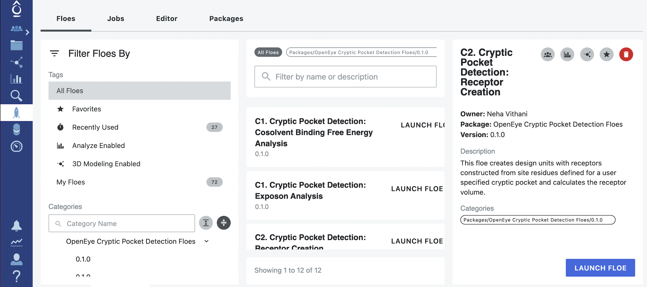
Start by clicking on the blue navigation side bar Floe tab. Click on the Floes tab at the top of the page and then filter for Packages -> OpenEye Cryptic Pocket Detection Floes. Select the C2. Cryptic Pocket Detection: Receptor Creation Floe and click the LAUNCH FLOE button.

Select the desired Output Path.

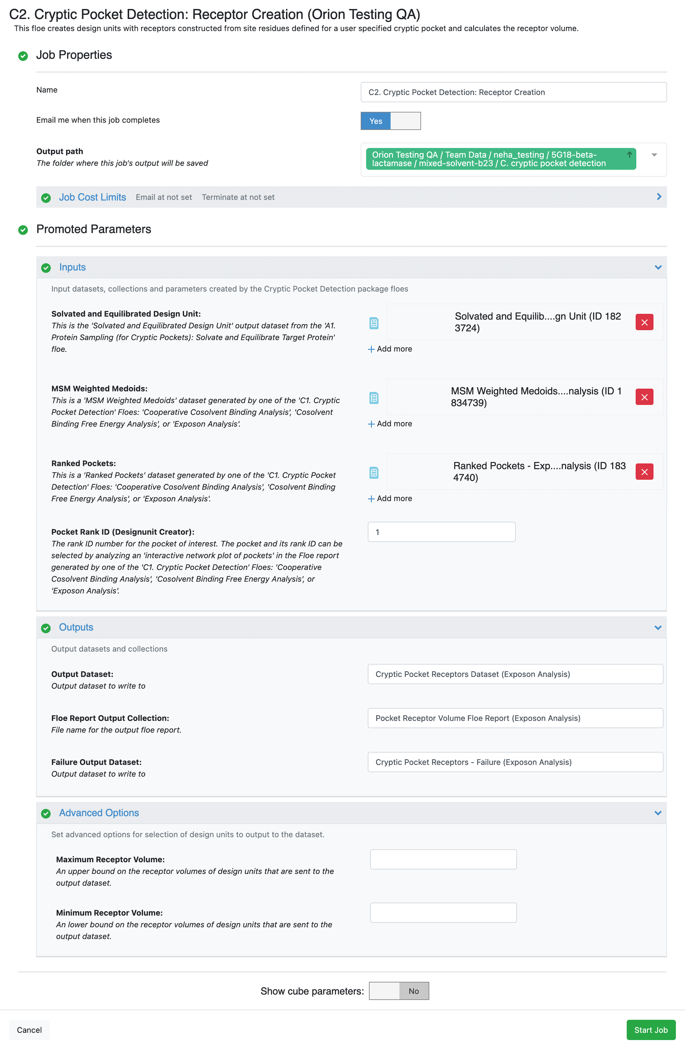
Provide the input files and parameters specified under the Inputs section. The input files required for this floe are those generated by running the A1. Protein Sampling (for Cryptic Pockets): Solvate and Equilibrate Target Protein Floe and the C1. Cryptic Pocket Detection: Cosolvent Binding Free Energy Analysis Floe.

• Solvated and Equilibrated Design Unit: Select the output design unit generated by the A1. Protein Sampling (for Cryptic Pockets): Solvate and Equilibrate Target Protein Floe. If you did not change the default output dataset name when running the floe, it will be Solvated and Equilibrated Design Unit.

• MSM Weighted Medoids: Select the MSM weighted medoids output dataset generated by the C1. Cryptic Pocket Detection: Cosolvent Binding Free Energy Analysis Floe. If you did not change the default output dataset name when running the floe, it will be MSM Weighted Medoids - Cosolvent Binding Free Energy Analysis.

• Ranked Pockets: Select the ranked pockets output dataset generated by the C1. Cryptic Pocket Detection: Cosolvent Binding Free Energy Analysis Floe. If you did not change the default output dataset name when running the floe, it will be Ranked Pockets - Cosolvent Binding Free Energy Analysis.

• Pocket Rank ID (Designunit Creator): Provide the rank ID number for the pocket of interest. The pocket and its rank ID can be selected by analyzing the interactive network plot of pockets in the floe report generated by the C1. Cryptic Pocket Detection: Cosolvent Binding Free Energy Analysis Floe.

Since this floe and its outputs do not depend on the type of pockets being analyzed, we recommend adding (Cosolvent Binding Free Energy Analysis) as a suffix to the default names given for the outputs: Cryptic Pocket Receptors Dataset, Pocket Receptor Volume Floe Report, and Cryptic Pocket Receptors - Failure.

Click on the green Start Job button at the bottom of the page.

Tip

Wait for the submitted job to finish. This floe will take up to three hours to finish and cost $4.

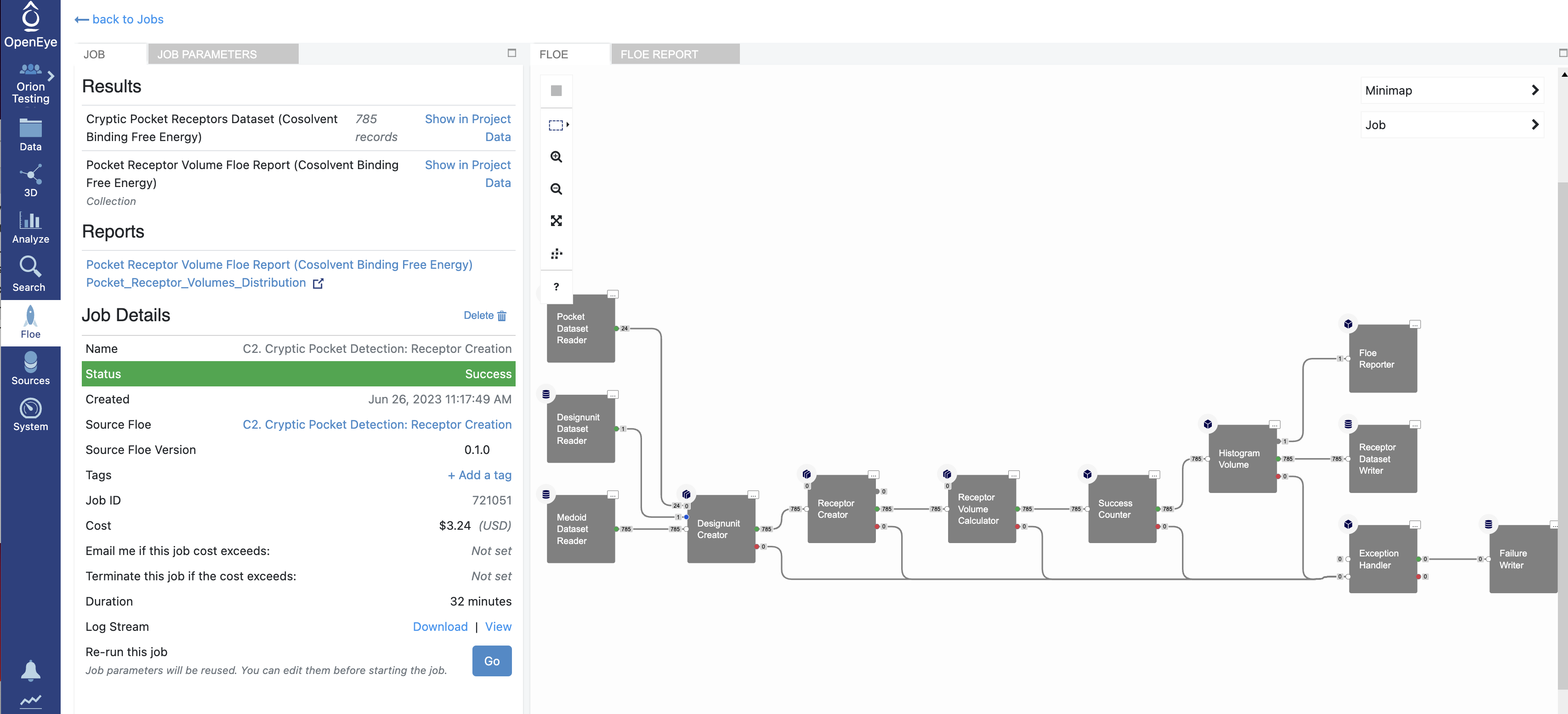
When the job is complete, the Pocket Receptor Volume Floe Report (Cosolvent Binding Free Energy Analysis) Pocket_Receptor_Volumes_Distribution and the Cryptic Pocket Receptors Dataset outputs should be inspected for visualization of pocket receptors and distribution of pocket volumes. You can get to this output by clicking on the job. Click on the Floe tab on the blue navigation side bar and then click on the Jobs tab at the top of the page. Next, click on the job that you want to inspect.

Under Reports, clicking on the Pocket Receptor Volume Floe Report (Cosolvent Binding Free Energy Analysis) Pocket_Receptor_Volumes_Distribution link will redirect you to a Pocket Receptor Volumes Distribution plot.

Click on this link floe report to download and visualize an example of the Pocket Receptor Volumes Distribution plot. This plot shows the distribution of pocket volumes for the selected pocket rank ID across representative conformations. Hovering over each data point in this plot will display the value of pocket receptor volume, the number of representative conformations with the given receptor volume, and their cumulative populations derived from Markov state modeling.

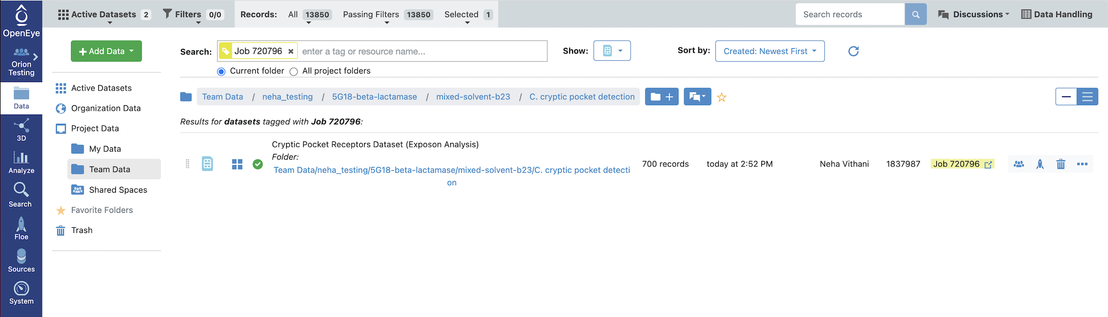
Under Results, click on Show in Project Data given next to the Cryptic Pocket Receptors Dataset to see the dataset associated with the job.

This will redirect you to the Data navigation side bar tab and show only the dataset associated with the job. Click on the icon of a blue circle with a + symbol that is next to the dataset name. It will change to a green circle with a white checkmark and will allow you to view the dataset in the Analyze and 3D Modeling pages.

Click on the navigation side bar Analyze tab. Make sure that your Active Dataset is set to Cryptic Pocket Receptors. On the scatter plot on the Analyze page, use the MSM Weight for the y-axis and Receptor Volume for the x-axis. Also click on the Layouts button in the top-right corner and select the Analyze with 3D option. This shows a visual representation of the protein structures of the representative conformations.

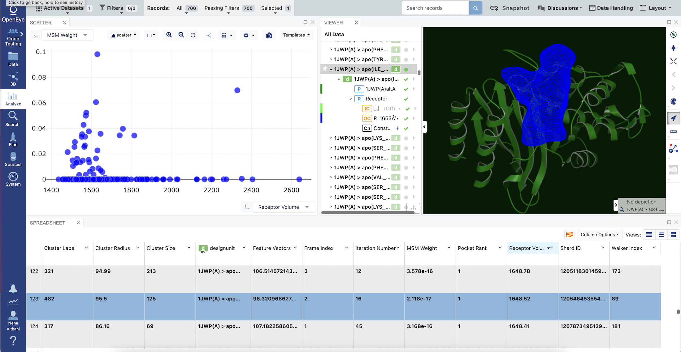
Clicking on the Receptor Volume column given in the SPREADSHEET sorts the representative conformations by the pocket receptor volumes in these conformations, in either ascending or descending order. After sorting the structures by volumes in the SPREADSHEET, click on a row with the Receptor Volume value of choice. This will display the protein structure in the Viewer panel corresponding to the selected row. Click on the small carrot next to the corresponding design unit listed under All Data to display all components present in this design unit. Click on Receptor, IC, and OC to visualize the receptor. The receptor will appear in blue-colored mesh. After visualizing different design units and their receptors, you can select an appropriate design unit for Gigadocking or Sitehopper Analysis.