Tutorial: Building Machine Learning Regression Models for Property Prediction of Small Molecules
OpenEye Model Building is a tool to build machine learning models that predict properties of small molecules.
In this tutorial, we will train several regression models to predict IC50 concentrations at which molecules become reactant to pyrrolamides. The training data is known as the pyrrolamides Dataset. The results will be visualized in both the analyze page and floe report. We will leverage the floe report to analyze and choose a good model. Finally, we will choose a built model to predict the property of some unseen molecules.
This tutorial uses the following Floe:
ML Build: Regression Model with Tuner using Fingerprints for Small Molecules.
Warning
This tutorial keeps default parameters and builds around 2.5k machine learning models. While the per model cost is very cheap, based on the size of dataset, total cost might be pricey. For instance, with the pyrrolamides dataset(~1k molecules) it costs around 100$. To understand the working of the floe, we suggest building lesser models by referring to the Cheaper and Faster Version of the tutorial.
Create a Tutorial Project
Note
If you have already created a Tutorial project you can re-use the existing one.
Log into Orion and click the home button at the top of the blue ribbon on the left of the Orion Interface. Then click on the ‘Create New Project’ button and in the pop up window enter Tutorial for the name of the project and click ‘Save’.
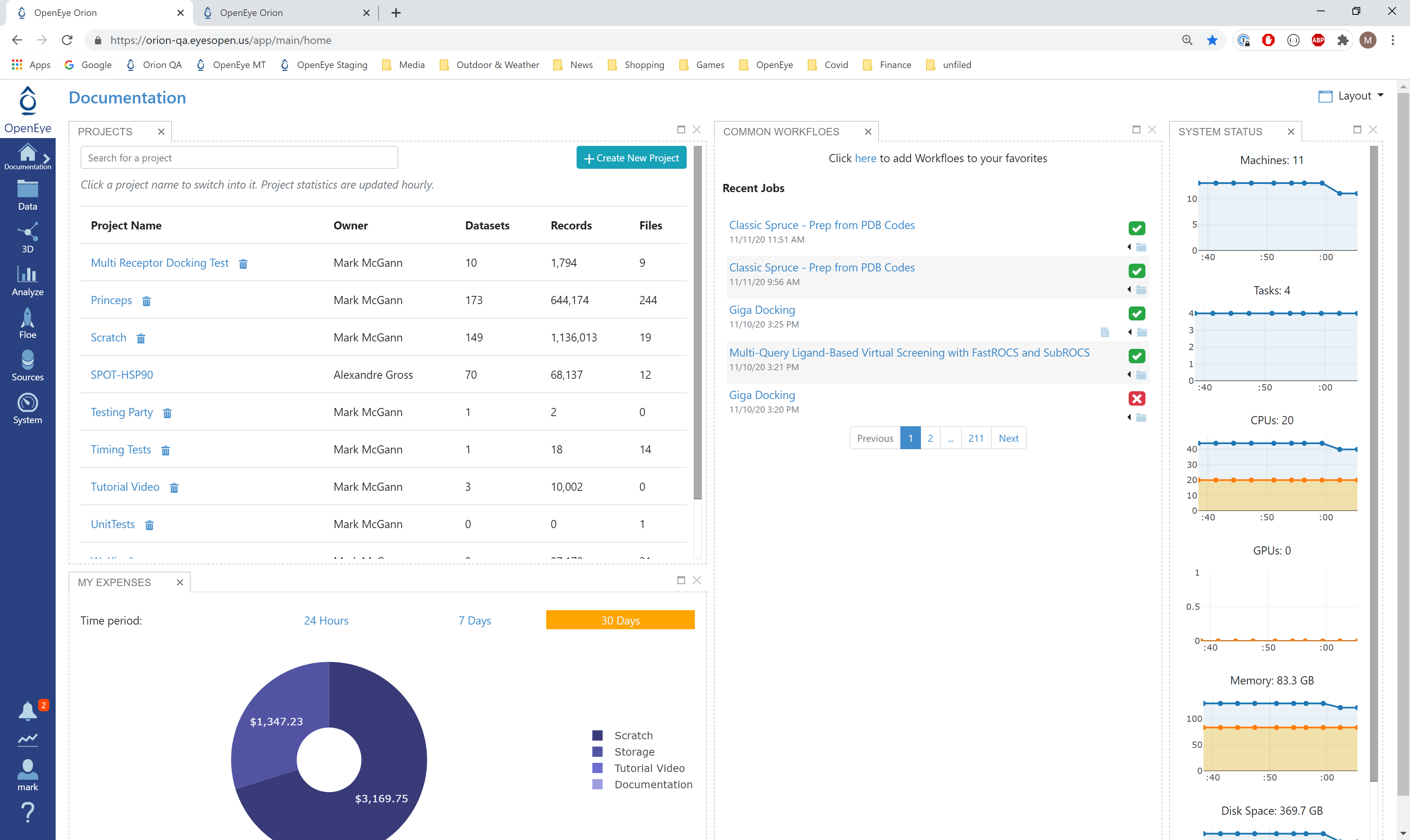
Orion home page
Floe Input
The Floe requires an input dataset file with each record in the file containing an OEMolField. Uploading .csv, .sdf or similar formats in Orion, automatically converts it to a dataset. There needs to be a separate field in each record containing the Float property to train the network on.
The Pyrrolamides dataset contains several OERecord (s). The floe expects two things from each record:
An OEMol which is the molecule to train the models on
A Float value which contains the regression property to be learnt. For this example, it is the IC50 concentration.
Here is a sample record from the dataset:
OERecord (
    *Molecule(Chem.Mol)* : c1ccc(c(c1)NC(=O)N)OC[C@H](CN2CCC3(CC2)Cc4cc(ccc4O3)Cl)O
    *NegIC50(Float)* : 3.04
)
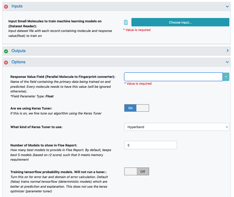
To start off, the input needs to be selected in the parameter Input Small Molecules to train machine learning models on.
We can change the default names of the Outputs or leave them as is.
The property to be trained on goes in the Response Value Field under the Options tab.
Input Data
Run OEModel Building Floe
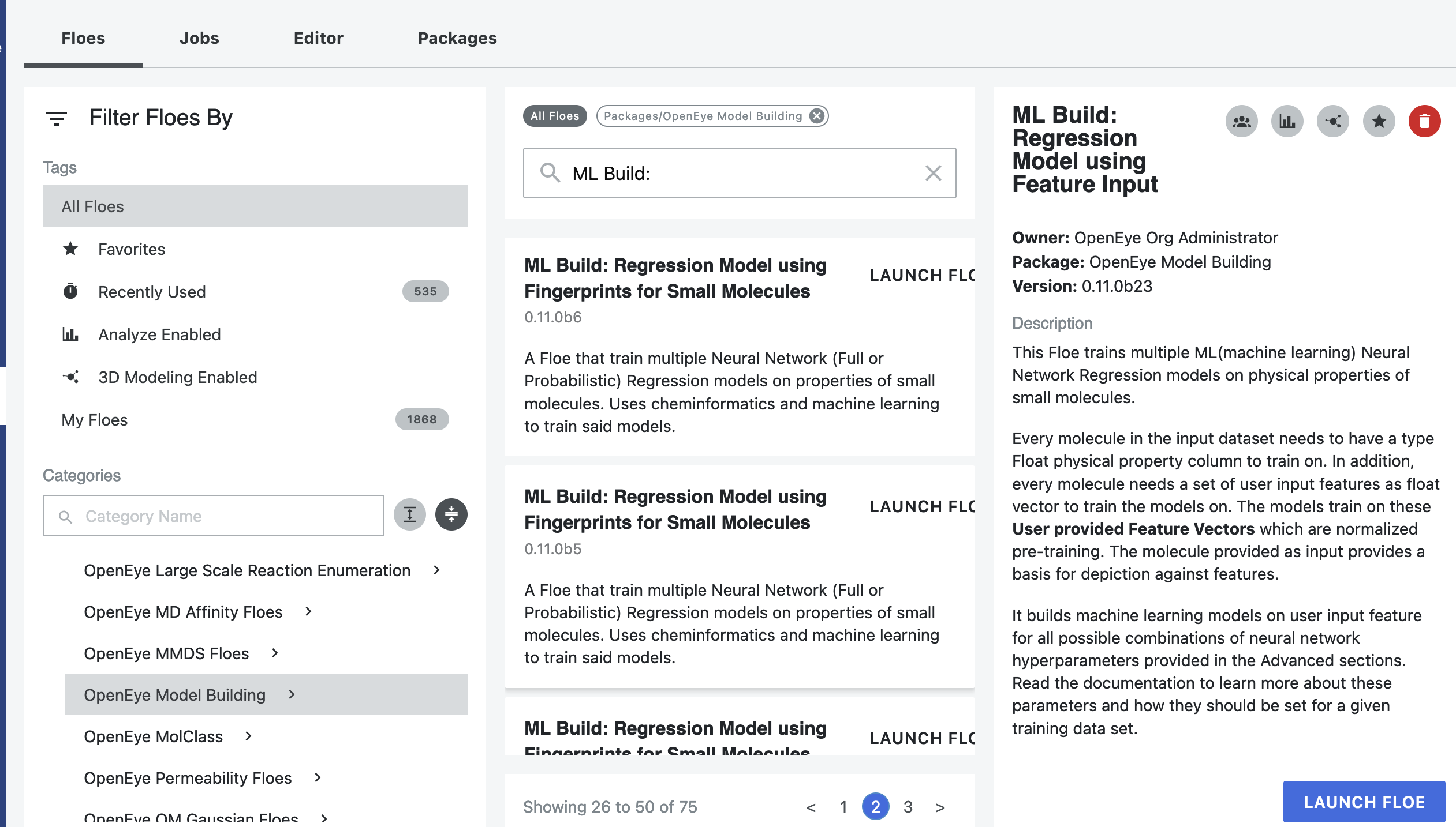
Click on the ‘Floes’ button in the left menu bar
Click on the ‘Floes’ tab
Under the ‘Categories’ tab select ‘OpenEye Model Building’ package
In the search bar enter ML Build
A list of Floes will now be visible to the right
Launch the floe ML Build: Regression Model with Tuner using Fingerprints for Small Molecules and a Job Form will pop up. Specify the following parameter settings in the Job Form.

Click on the Input Small Molecules to train machine learning models on. button
Select the given dataset or your own dataset.
Change the name of the ML models built to be saved in Orion. We will keep it to defaults for this tutorial.
Select the response value which the model will train on under the Options tab. This field dynamically generates a list of columns to choose from based on the upload column. For our data, its NegIC50.
Promoted parameter Are we using Keras tuner: Uses Hyperparameter optimizer using Keras Tuner. Keep this on by default
Promoted parameter What kind of keras tuner to use: You can keep Hyperband by default or change to any of the other options.
Select how many model reports you want to see in the final floe report. This fields prevents memory blowup in case you generate >1k models. In such cases viewing the top 20-50 models should suffice.
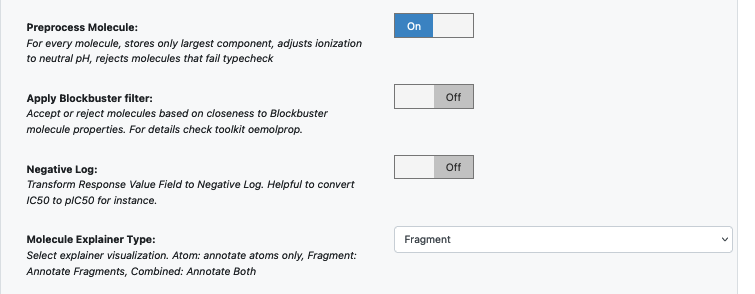
Promoted parameter Preprocess Molecule :
Keeps the largest molecule if more than one present in a record.
Sets pH value to neutral.
You can apply the Blockbuster Filter if need be
In case it is necessary to transform the training values (Pyrrolamides in this case) to negative log, turn the Log. Neg Signal switch as well. Keep it off for this example.
Select how you want to view the molecule explainer for machine learning results.
‘Atom’ annotates every atom by their degree of contribution towards final result.
‘Fragment’ does this for every molecule fragments (generated by the OEMedChem tookit) and is the preferred method of med chemists.
‘Combined’ produces visualizations of both these techniques combined.
You can let the model run at this point and it should run with default parameters. But we can tweak a few parameters to learn more about the functionality.
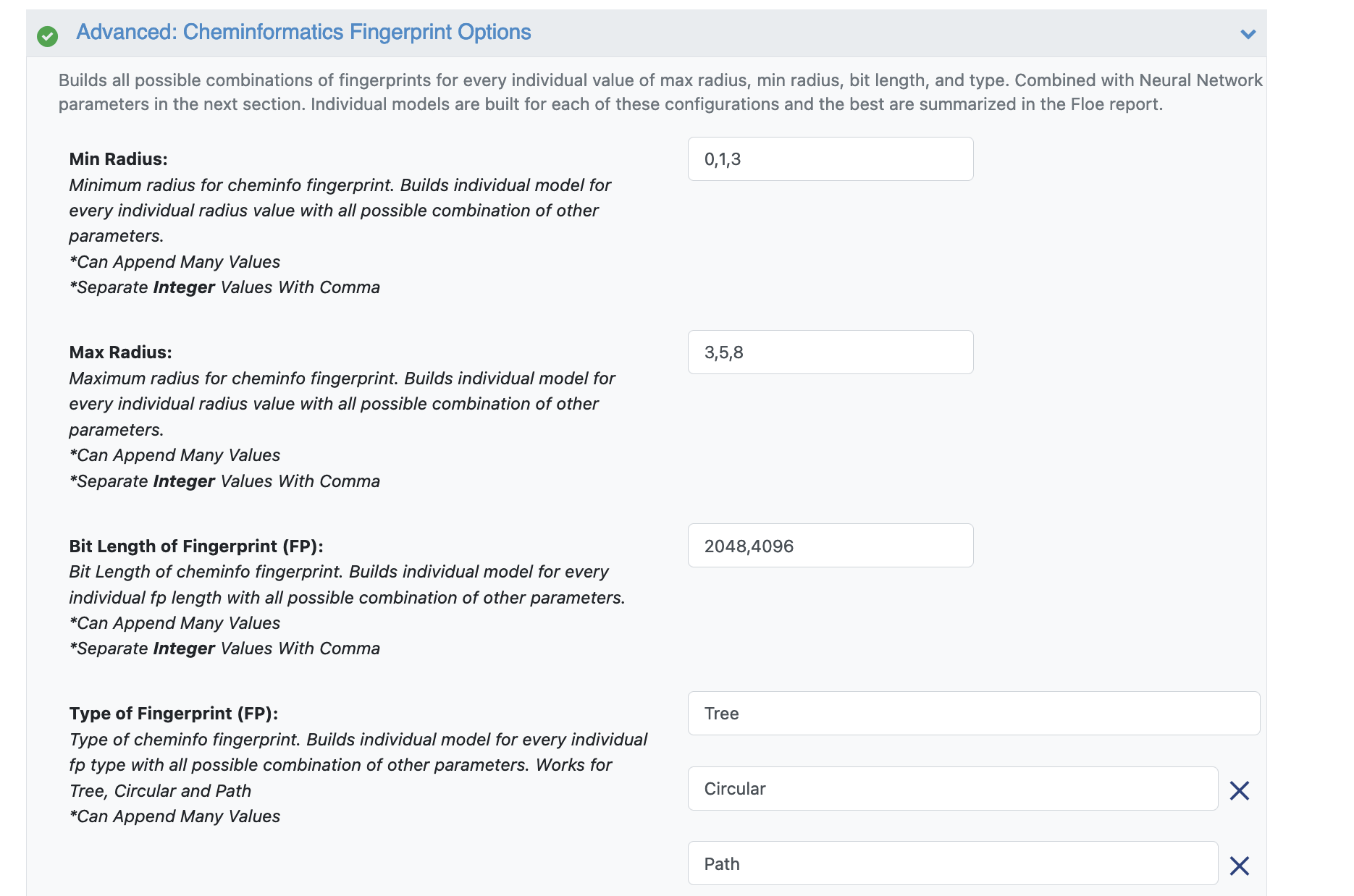
Open the Advanced: Cheminfo Fingerprint Options. This tab has all the cheminformatics parameters the model will be built on. We can add more values to the fingerprint parameters as shown in the image. Feel free to add other parameter values and play around as well.
For suggestions on tweaking, read the How-to-Guide on building Optimal Models
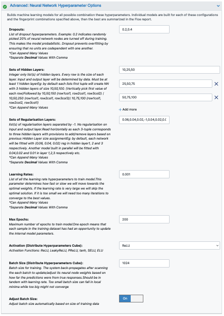
Next we move to the Advanced: Neural Network Hyperparameters Options. This is where the Machine Learning parameters are listed. Again, we can leave them to defaults, or choose to add/modify a few values based on the How-To Guide.
We add dropout to further prevent overfitting.
Next, let us inspect the parameter Sets of Hidden Layers. Every row is the node size of each layer. Each node from each layer is combined with another from the next to create an ML model. By default there are three 3-layer networks. Plugging in the formula stated in the How-to Guide (building Optimal Models), we should probably reduce the number of nodes to prevent overfitting. Change Layer1 to 10,25,100. Layer2 to 20, 50, 75. Layer3 can be changed to 50, 75, 100.
Another important hyperparameter listed next is the regularization. This field sets L2 regularization for each network layer, making it a -1 separated 3-tuple list as well.
Increasing the Learning Rate is a way of speeding things up, although the algorithm may not detect the minima if this value is too high. We can train our model on multiple learning rate values. Leave defaults here.
If the dataset is big, we may consider increasing the epoch size as it may take the algorithm longer to converge. Leave defaults here.
Activation: Relu is probably the most commonly used activation function for most models. Change to one of the options in the list (see How-to-Guide on building Optimal Models)
The Batch Size defines the number of samples that will be propagated through the network. With larger batch there is a significant degradation in the quality of the model, as measured by its ability to generalize. However, too small of a batch size may take the model a very long time to converge. For a dataset size of ~2k, 64 is probably a good batch size. However for datasets of size say 100k, we may want to increase batch size to at least 5k.
Set Batch size to 64
Lastly, Neural Network Ensemble Size determines how many models per run will be trained and provides a robust confidence interval.
That’s it! Lets go ahead and run the Floe!
Analysis of Output and Floe Report
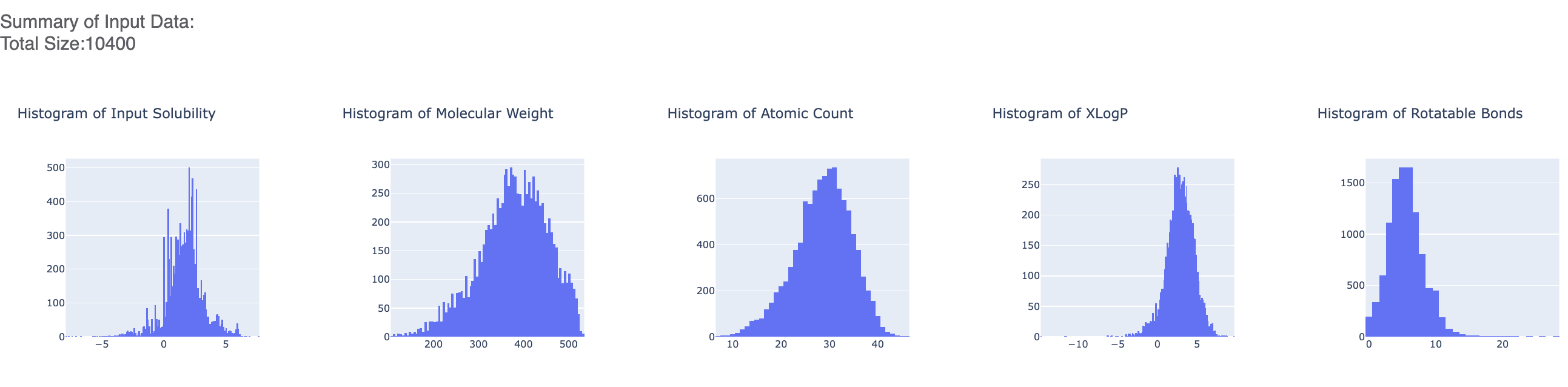
After the floe has finished running, click the link on the ‘Floe Report’ tab in your window to preview the report. Since the report is big, it may take a while to load. Try refreshing or popping the report to a new window (located in the purple circle in the image below) if this is the case. All results reported in the Floe report are on the validation data. The top part summarizes statistics on the whole input data.
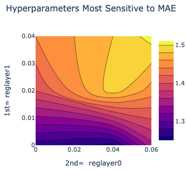
The graphs show the Mean Absolute Error (MAE) for different values of the neural network hyperparameters. It helps us analyze how sensitive the different hyperparameter values are and plan future model builds accordingly. For instance, graph below shows that dropout of 0.1 and maxr of 5 are better choice for parameters in future model build runs.
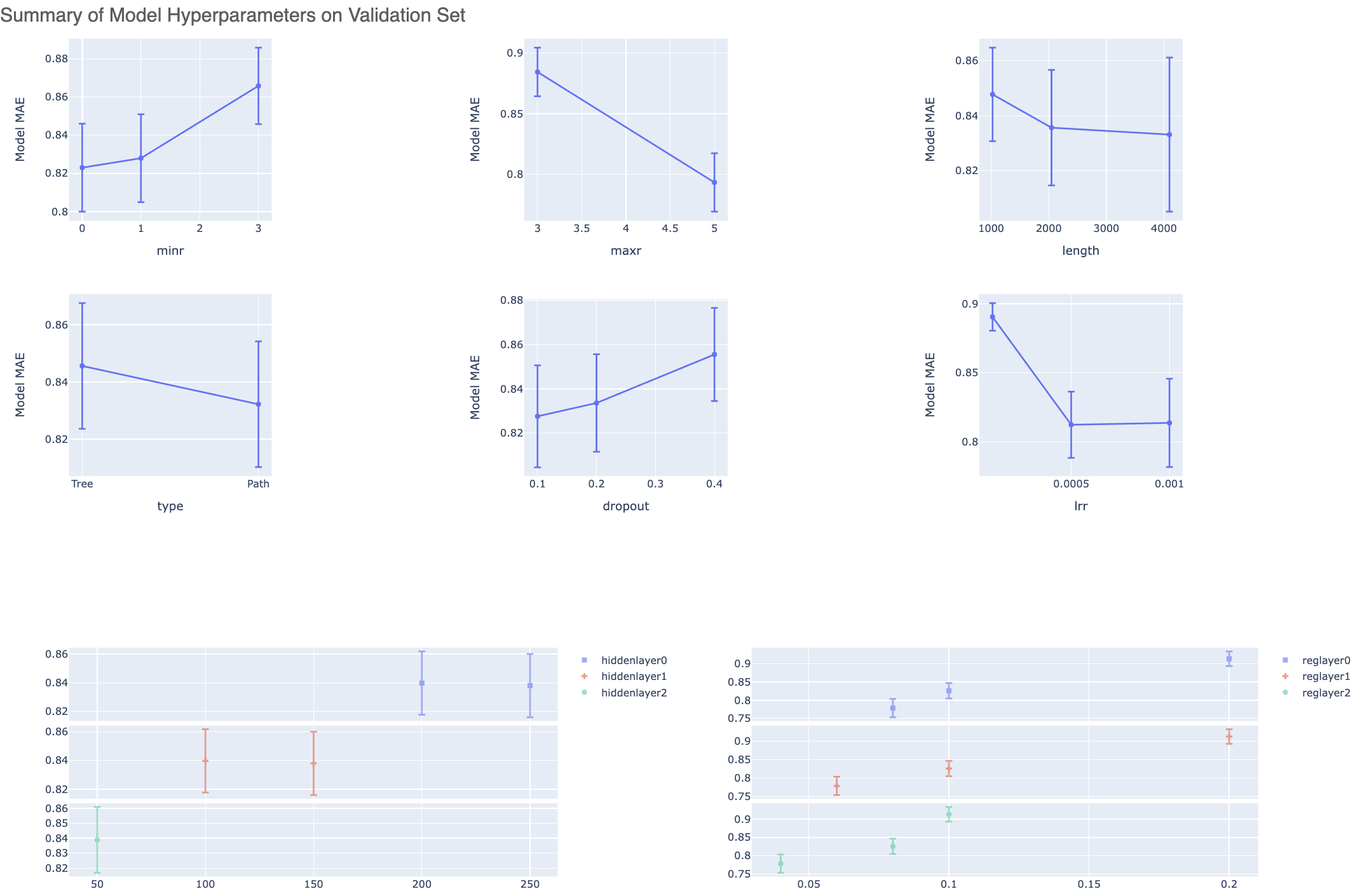
There is also a plot between the top two most sensitive hyperparameters. Therefore we can choose these parameter values to be near to wherever the least MAE is in the heatmap.
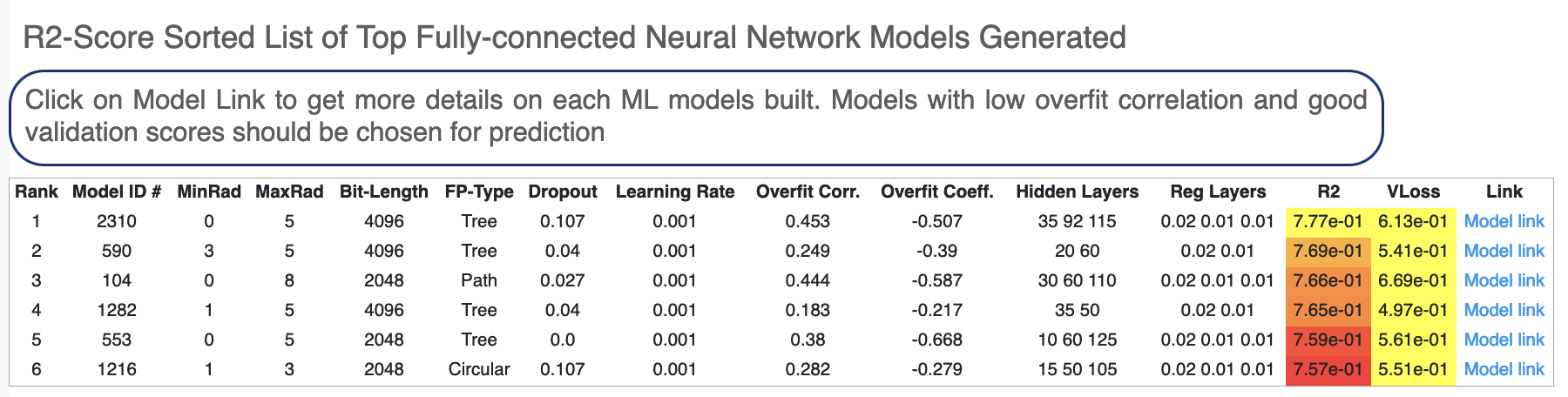
Next, we tabulate the list of all models built by the fully connected network. These models are sorted by the least R2 Score (for validation data). On the face of it, the first row should be the best model since it has the least error on the validation data. But there can several other factors besides the best R2 to determine this, starting with Loss in the next column. Hence, lets look at a sample model by clicking the ‘Model Link’. Let’s click on a model link and look at the training curves under ‘Neural Network Hyperparam and Fingerprint Parameters’.
For each model, we have a linear color scale showing the rank. We also have the cheminformatics and machine learning parameters the model was trained on.
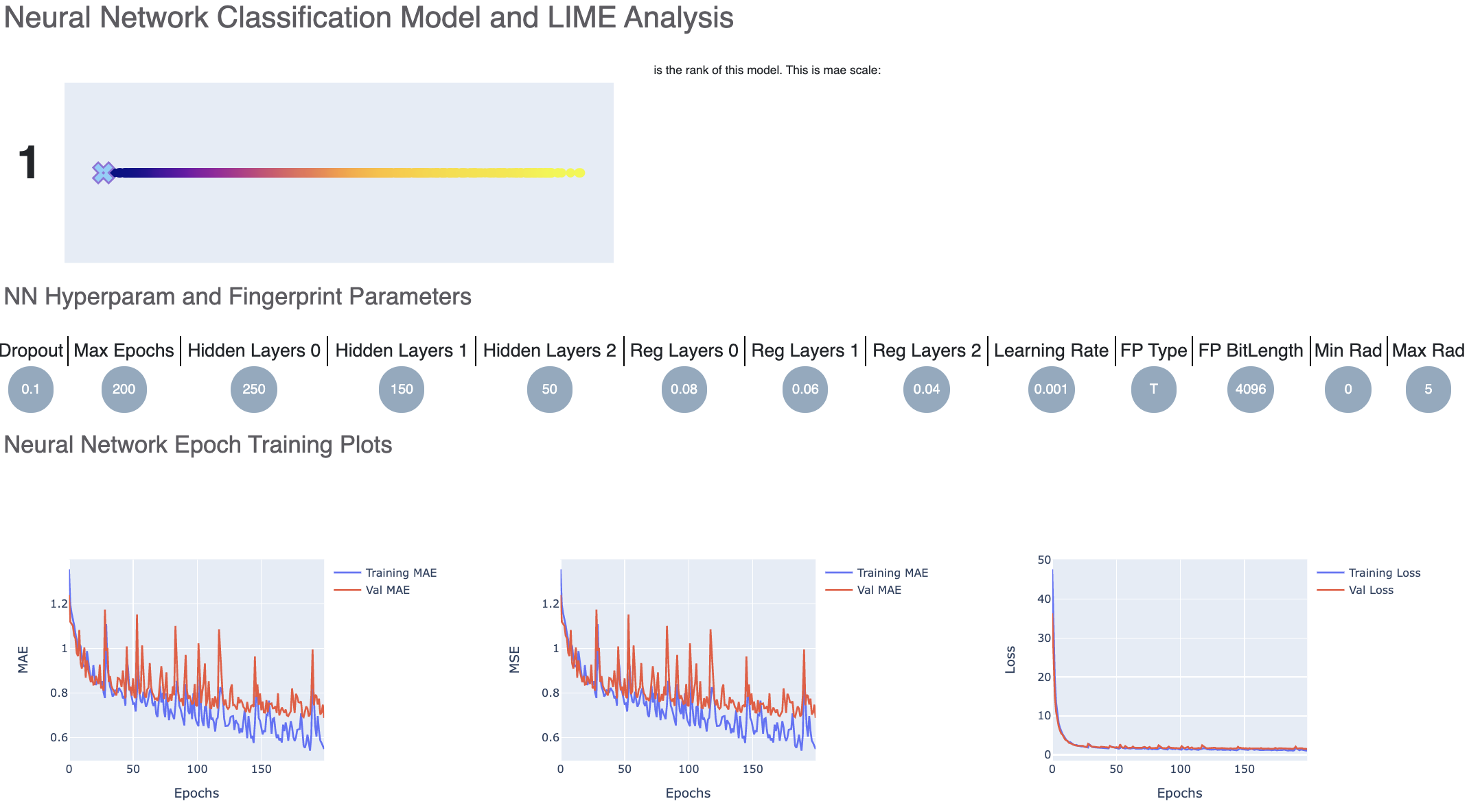
We see that the training and validation MAE follow similar trend which is a good sign of not overfitting. Had they been diverging, we might have to go back and tweak parameters such as number of hidden layer nodes, dropouts, regularizers etc. Although too much fluctuation in the graph suggests we need a slower learning rate.
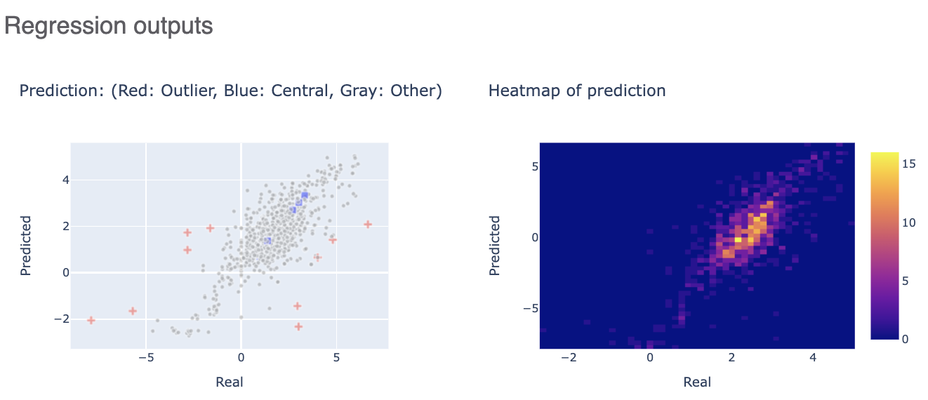
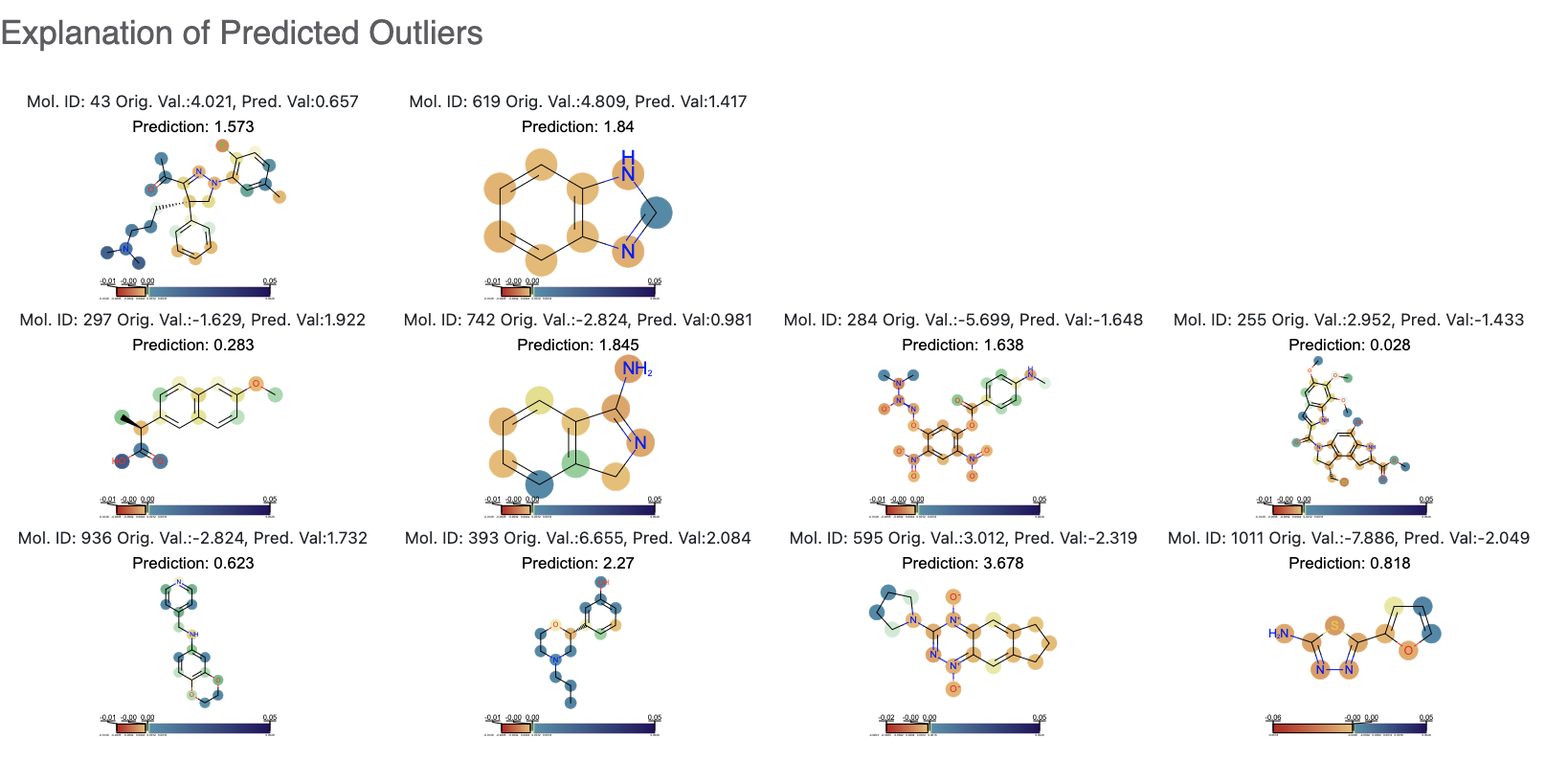
The Regression output plots real versus predicted to show how well the training is correlated. Below that, click on the interesting molecule to see the annotated explainer of the machine learning model.
While this tutorial shows how to build regression models, building an optimizing one is a non-trivial task. Refer to the How-to Guide on how to optimize model building based on the data available.
After we have found a model choice, we can use it to predict and or validate against unseen molecules. Go to the next tutorial Use Pretrained Model to predict generic property of molecules to do this.