POSIT Theory
Overview
OEDocking’s POSIT is pose-prediction tool primarily based on the assumption that similar ligands bind similarly. Pose prediction is the process of determining the structure of a ligand bound in the active site of a target protein. OEDocking’s POSIT method of pose prediction consists of choosing the best method to use when docking a particular ligand to a receptor and then returning the probability that the docked pose is within 2.0 Ångströms of the actual pose. The posit application returns the pose with the highest probability of being correctly placed in the active site assuming that the molecule actually binds to the given protein. The known bound ligand is used to impart docking constraints when placing and optimizing the geometry of the molecule being docked.
Note
This probability is not the probability of binding, it is the probability that the pose is correct given the ligand actually binds to the receptor.
The methods current posit uses to dock are, in order of preference:
MCS Overlay [Hare-2004] - Maximum Common Substructure overlay followed by a shape-guided minimization into the receptor site.
ShapeFit - Shape-guided ligand minimization into the receptor site
HYBRID - hybrid method that uses ligand and protein information
FRED - Standard docking method that uses no ligand information
posit automatically chooses the best method based on the 2D (graph) and 3D (structure) similarity of the docked ligand to the bound ligand. As a contrived example, if there is no bound ligand in the receptor, the FRED method is used by default. posit attempts to use as much ligand information as possible. For example the results of the ShapeFit overlay can be seen in SHAPEFIT Cross Docking Results.
posit’s first pass is to identify a target receptor that has the most similar bound ligand. Multiple receptors are not required, but increase the odds of posit finding a suitable receptor. Given an input molecule, posit identifies the most similar bound ligand using a combination of graph similarity to the bound ligand (MACCS 166 set or OpenEye’s PATH fingerprints) and 3D similarity, TanimotoCombo, to the bound ligand.
These similarities have been calibrated to produce a probability of predicting a pose within 2.0 Ångströms RMSD.
By default, in addition to the input conformations, posit generates new conformations during its search and, in some cases, minimizes these structures with the internal force-field.
TanimotoCombo
posit uses the TanimotoCombo measure to compare (and optimize) predicted and bound ligands. The TanimotoCombo measure is simply two separate Tanimoto measures added together. While most uses of Tanimoto have been to compare fingerprints together, there is a direct relation between the 1D fingerprint bit vector and 3D space:
The basic equation for a field Tanimoto between two fields A and B is:
In the case of posit, the field in question can be thought of as field of voxel space. For \(Tanimoto_{shape}\), where A and B are now molecules: if two objects fill the same voxels, then the Tanimoto value is 1.0. If two objects don’t overlap by half, the Tanimoto value is 0.5 and so on. (The term voxel is used for purposes edification, in actuality the volumes estimated using a fast approximate method)
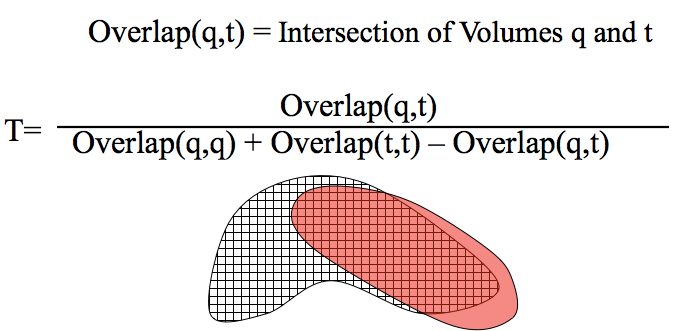
Voxel Representation of Shape: Similar to fingerprint bits in 1D, voxels can be used to represent 3D space and compared with the Tanimoto measure. The numerator Overlap(q,t) is essentially the volume of the intersection of q and t and the denominator Overlap(q,q) + Overlap(t,t) - Overlap(q,t) is essentially the volume of the union of q and t.
The field can also contain colored representations of chemistry. For example, if two voxels are colored as hydrogen bond donors and overlap, the \(Tanimoto_{color}\) increases.
Hence, TanimotoCombo is:
TanimotoCombo values range from 0 (no overlap) to 2.0 (full shape overlap and full color or chemistry overlap).
A note on stereo - isomerisms and chirality
Stereo, and notably nitrogen aniline stereocenters, are currently somewhat problematic for posit. Many crystal structures have flat geometries for some stereocenters due to time-averaging during data collection. This makes stereocenters appear to have flat geometries in the 3D coordinates.
Note
By default posit ignores stereo on nitrogen bases. While this can be problematic for some structures, because posit can optimize toward a bound ligand, this is ameliorated somewhat. Please see the posit usage section for how to turn this off.
posit automatically enumerates missing stereo (except for nitrogen base stereo as described above). Because the POSIT algorithm internally expands conformations during the flexible fitting procedure the full molecule must be labeled with stereo, either in the 3D coordinate sense or the 2D coordinate sense.
The recommended way to run posit is to start with an existing database of conformations. Use OMEGA or the OMEGA toolkit to prepare molecules or expand the stereo chemistry using OEFlipper. posit is guaranteed to work correctly if the input molecules have been generated by OMEGA.
Note
Structures output by posit are not guaranteed to have the same conformations of the input molecule. This is occasionally problematic if the force-field minimizations alter the desired input conformations, for example taking a planar nitrogen and forcing it into a stereo conformation.
POSIT Algorithm
posit supplies a robust probability that the given pose is reasonable. It is generally recognized that docking and scoring methods have inaccuracies and do not provide a measure that can be compared between different complexes. For example, a docking score from one complex cannot be directly compared to a docking score form another.
posit overcomes this by using 2D, 3D and protein-ligand information to generate a probability that the pose has been correctly placed. This probability is independent of how the ligand was actually placed and hence, can be used to score any prospective pose. Indeed, the ShapeFit method was explicitly designed to maximize this probability.
posit probabilities were generated using a large test set containing over 25,000 pose predictions and verified through a smaller number (around 100) of predictions that were then validated with X-Ray crystallography. It is important to note that posit does not give a probability of binding, rather it gives a probability that if the ligand does actually bind, what is the likelihood of the posit pose being the actual pose.
ShapeFit Method
During a drug discovery campaign, thousands of small molecule inhibitors are made in the course of optimizing molecular properties. For projects that have X-Ray crystallographic (XRC) coordinates, structure-based designs help guide the medicinal chemistry efforts. In many cases XRC provides a detailed picture of the binding of a small-molecule inhibitor into the binding site.
Many techniques exist for pose-prediction and are well documented [Erickson-2004] . However, very few provide a probability that the generated pose is correct, where correct is typically considered to be less than 2.0 Ångströms RMSD (root mean square distance) from experimental crystal structure. In fact, many docking scores such as Chemscore, Chemgauss3, PLP [Tuccinardi-2010] are not very correlated with correct ligand pose, and worse, are not transferable between systems: the best docking score in one system may not even be close to the best docking score in another.
Two definitions will be used during the remainder of this discussion:
Bound-Ligand This is a known, experimentally derived bound ligand from the same protein context in which SHAPEFIT is attempting to find poses of ligands.
Fit-Ligand This is the unknown ligand that is being pose-predicted.
Using the Bound Ligand
SHAPEFIT overcomes these issues by comparing predicted poses to observed bound ligands in related co-crystals. As the observed ligand becomes more similar to the predicted pose, both the binding mode and, indeed, the shape of the receptor pocket itself tends to become more similar.
The similarity measures being used are 2D path-based fingerprints and the 3D TanimotoCombo [Hawkins-2010] that compares shape and the Mills-Dean approximation of electrostatics [MillsDean-1996] . These similarity measures choose the most appropriate system to dock against and provide a prediction of the quality of the result.
The TanimotoCombo measure is agnostic of how the poses in question are generated; it can be used to validate and provide a pose prediction probability regardless of how the pose was generated. In practice, SHAPEFIT exploits the predictive capabilities of the TanimotoCombo measure by using it in an optimization function that drives a flexible fitting routine.
Essentially, during pose optimization, SHAPEFIT attempts to force a predicted pose into the binding mode of a known ligand. If the induced strain becomes too large, the optimization stops. This final pose is used to predict the overall quality of fit. In this fashion, SHAPEFIT is able to rescue 10-20% of the original rigidly overlaid poses and place them within 2.0 Ångströms RMSD of the experimental crystal structure.
Typically during docking, only the protein structure is used to model unknown structures. Given a molecule that is known to bind, SHAPEFIT searches through XRC coordinates of known ligand-protein complexes, determines the complex best able to predict the pose of the molecule and then generates both a pose and the probability that the pose is correct, usually in well under a minute per ligand.
SHAPEFIT’s basic algorithm:
Given a set of potential complexes, SHAPEFIT chooses the appropriate complex based on the 2D or 3D similarity to the bound ligand. The best complex, in general, has the highest 2D or 3D similarity of the input molecule to the chosen complex’s bound ligand.
After the complex is chosen, a flexible fit is performed that attempts to match the binding mode of the bound ligand using an adiabatic optimization method [Wlodek-2006] . This optimization method is known as the SHAPEFIT potential.
The term adiabatic comes from the Greek “impassable”, and in this case SHAPEFIT sets up a chemical strain boundary that the optimization cannot broach.
SHAPEFIT seeds the flexible fit by expanding the poses generated by the original 3D similarity as described in (1) and then applying the shape constraint of the bound ligand.
As shown in figure SHAPEFIT Optimization, SHAPEFIT works by first using the known bound ligand to position the input molecule and follows up by using the bound ligand as a shape constraint during MMFF optimization [Halgren-I-1996] [Halgren-II-1996] [Halgren-III-1996] [Halgren-IV-1996] [Halgren-V-1996] [Halgren-VI-1999] [Halgren-VII-1999] . While the input molecule is being forced into the shape constraint, MMFF strain is monitored to form the adiabatic boundary. When the strain becomes too large, the optimization is reversed or stops altogether.
The interactions from the bound ligand are then used as a further constraint during ligand-protein optimization. This helps to remove clashes with the protein and provide better interactions between un-constrained ligand atoms.
This is a long winded way of saying that SHAPEFIT’s optimization attempts to force the molecule into the known binding mode without creating undue strain on the molecule being placed into the protein.
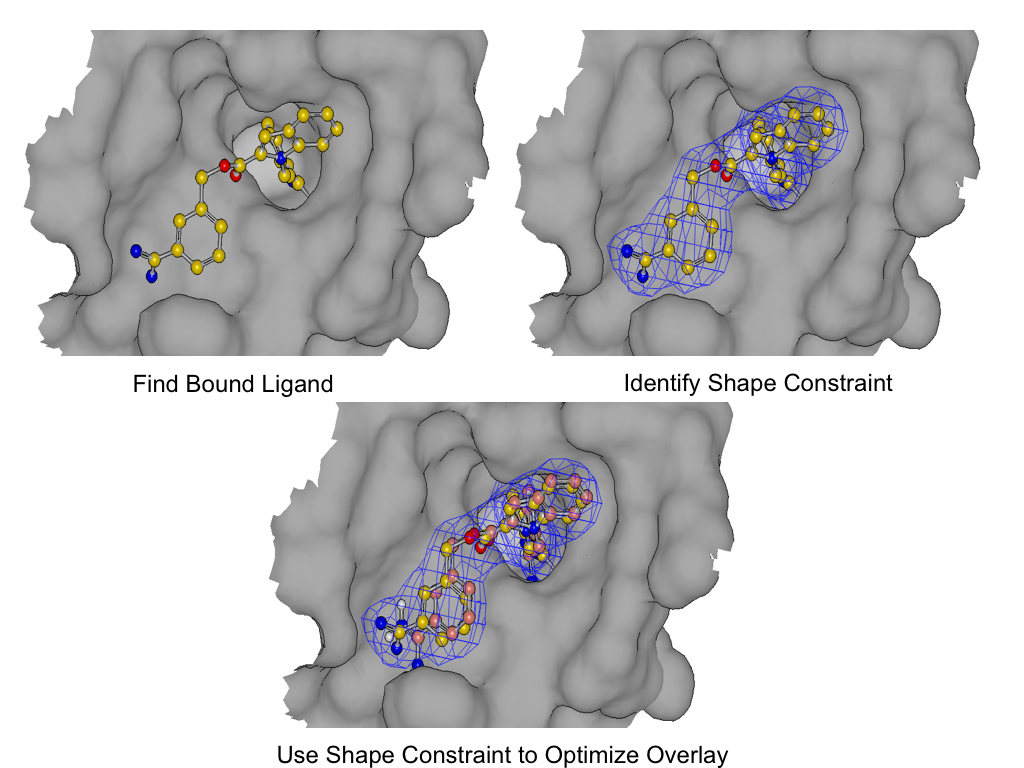
SHAPEFIT Optimization: Starting from an initial alignment, use the shape constraint of the bound-ligand to drive a flexible fit while simultaneously limiting strain
As shown in figure SHAPEFIT Cross Docking Results, analyzing the Kinase data set used in Tuccinardi et al, [Tuccinardi-2010] pose-prediction using SHAPEFIT is seen to perform remarkably better for similar ligands than standard docking techniques at higher TanimotoCombo values:
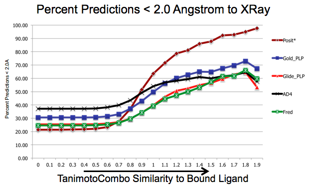
SHAPEFIT Cross Docking Results: Probability of finding a good pose based on bound-ligand fit-ligand TanimotoCombo similarity. Standard docking results are essentially the same and follow the same trajectories flattening out as they hit their limit of accuracy. While SHAPEFIT performs worse at low similarities it continually increases as similarity increases.
While SHAPEFIT is not a good technique for determining the pose between known bound-ligands and fit ligands with low similarity, as the similarity increases, the probability of determining the correct pose increases rapidly. The similarity where this crosses over is remarkably small, only around 0.9 TanimotoCombo. This is most likely because as the similarity increases, the active site similarity also increases. Below 0.9 TanimotoCombo posit reverts to the Hybrid method.
Predicting the Quality of the Pose
posit uses a robust measure of shape and chemical similarity to provide a probability of the generating the correct pose. Again, the definition used for correct is a pose less than 2.0 Ångströms to the experimental crystal structure.
Using a combination of public data and proprietary data obtained experimentally from collaborators, basic descriptors of 2D and 3D similarity between the ligand being fit and known bound ligands were analyzed to provide a basis for predicting the likelihood of obtaining a docked pose within 2.0 Ångströms when using a known target receptor as the docking target.
Figure POSIT Probability MAP shows how the beliefs given by the 2D and 3D measures are combined into a probability of having a good pose. Remember that this probability has been generated from ligands that actually bind, hence, it is not a probability of binding.
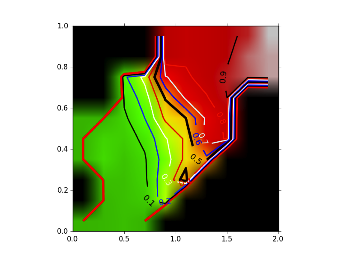
POSIT Probability Map: Given a 2D similarity (in this case the MACCS 166 descriptor set) and a 3D similarity (TanimotoCombo) posit computes a probability of finding the correct pose based on an analysis of historical and experimental data.
Note
This measure is independent of the technique used for posing, i.e. if a pose docked by the OEDocking tool FRED and produces a high TanimotoCombo to the known crystal structure, the probability of being the correct pose is the same as it would have been with posit.
This result is different from the result shown in [Tuccinardi-2010] , where they reported that having a high TanimotoCombo to the known bound ligand did not dramatically increase the quality of the resulting pose (even for FRED). The reason is subtle: Tuccinardi et al were computing the highest TanimotoCombo that the two molecules could obtain, while posit computes the actual, docked, in-place TanimotoCombo of the fitted pose. That is, if the docking algorithm produces an alignment of fit molecule to known bound ligand that overlaps with a given TanimotoCombo, one can look up the probability the docking was successful. In point of fact, posit is specifically designed so that the docked pose obtains the highest TanimotoCombo score possible while simultaneously minimizing induced strain and maintaining interactions with the protein.
Using the data shown in POSIT Probability MAP, for each pose, posit reports a simple score for the quality of the pose. The probability of a good pose is binned into the following results:
Result
Meaning
GREAT
Computed pose is likely (75%-100%) probability) to be within 2.0 Å of experimentally-derived pose.
GOOD
Computed pose may be (50%-75%) probability) to be within 2.0 Å of experimentally-derived pose.
MEDIOCRE
Take with a grain of salt (33%-50%) probability)
POOR
Take with a huge grain of salt (<33% probability)
By default, posit only outputs poses that are GOOD or better or that have a probability greater than or equal to 50% of being correct.
Poses that clash with the reference protein are not output. Both of these properties, probability and clash distance, can be tailored to individual preferences.
Additional Constraints (MCS)
Walter’s et al noted that a large portion of ligands bound to the same protein kinase share a large maximum common substructure (MCS). This was the basis for their CORES algorithm [Hare-2004] . posit can optionally identify matching regions and use them as additional constraints during optimization.
By default, posit searches for an MCS match to the bound ligand. The matching portion is used as the shape constraint, the rest is optimized against the protein.
On Clashes
The definition of clashes is somewhat problematic for purposes of pose prediction. In general, serious clashes where interpenetration with the protein should be avoided at all costs. However, when docking into a rigid protein that does not have the appropriate conformation, rigid docking ignores that fact that the active site may adopt a conformation suitable to the posed ligand.
The posit application deals with clashes by allowing the user to specify three allowable clash levels with cutoffs taken by analyzing various ligands in deposited in the protein data bank (PDB).
Allowed Clash
Description
noclashes
No clashes are allowed. Actually there is a little wiggle room here less than 0.2 Ångström penetration is not considered a clash.
mildclashes
Mild clashes are allowed ( >= 0.2 Ångström < 0.65 Ångström interpenetration)
allclashes
All clashes are allowed.
If a pose clashes, it is not thrown away, it is written to the clashed molecule file. Clashed molecule files hold ligands with decent probability when compared to the bound ligand, but have unallowable clashes with the protein.
Clashing can also affect the known bound ligand. When making a receptor for posit, if a bound ligand clashes with the protein beyond the allowable clash level, a warning will be given and the receptor will not be generated. In this case, the appropriate command line switch will be given in order to generate the receptor. It is advisable to visually inspect clashing complexes (and electron density if available) to decide whether the clash is acceptable or not.
Note that if a receptor is made with the -allclashes option, posit
should also be run with the same option or the -clash file should
be specified on the command line.
Unlike the FRED and HYBRID methods, SHAPEFIT is heavily biased towards the known bound ligand. In some cases this causes the pose to clash with the protein. This is especially true if the original bound ligand already clashes with the protein.
Currently, we do not filter out clashing poses although options and functionality for controlling this with SHAPEFIT will be investigated in future releases.