Philosophy and Design
We all care about water. It is the one thing we always need to take into account and it’s also the one thing we have most trouble modeling. A recent historical review of theories of water lists over thirty different models [Guillot-2002], none of which are comprehensive in their predictive abilities, i.e. are able to reproduce all of water’s many properties. However, we really don’t care about the thermal conductivity or viscosity of water, we just want to know how it interacts with solutes of interest, typically a drug molecule and a protein. Here, simple atomistic modeling of water ought to be adequate. And for very simple molecules, e.g. alkanes, mono-functional substituted alkanes, simple aromatics, all-atom simulations can appear to be capturing interactions between water and the solute quite well, for instance in predicting the transfer energy from vacuum to water. However, attempts to predict such energies on more complicated molecules are much less accurate and, what is worse, appear to be no better than a simplistic approach such as Poisson-Boltzmann (PB) [Nicholls-2008], [Nicholls-2009]. In PB we model water not atomistically but as a continuum, as a high dielectric that responds to the potential produced by the solute. PB cannot account for the van der Waals interactions between water and the solute other than by some simple area term and cannot account for discrete water effects, hydrogen-bonding patterns or correlation between waters. All it can do is to present an effective response, a long-time response if you will, of a material that macroscopically acts like water in its dielectric response. Yet PB continues to prove useful and predictive, presumably because the behavior it does model is the dominant behavior for interaction energetics and because many of the aspects of water claimed to be important either are not or cancel each other in some poorly understood manner. An example of this was discovered early in PB theory, namely that of the results for highly charged ions, where water structure was presumed to be absolutely necessary for prediction. Closer study illuminated two effects: electrostriction, causing water density to be higher near the ion, and dielectric saturation, i.e. the field of the ion so aligns water that it no longer responds linearly to that field. These two effects act to cancel each other—electrostriction increases the effective dielectric while saturation decreases it. As a consequence, PB is quite accurate for highly charged ions.
Despite the fact that all-atom simulations have proven quite poor at predicting the energies of anything but simple molecules (e.g. RMS error of \(\sim \, 2 \, kcal \, mol^{-1}\)) they are routinely applied to the much more complicated task of active site modeling. It is natural to try such techniques because this is the area of interest for drug discovery and, to be fair, the solvation of simple amino acids is well understood. It is also felt that simulations must be more useful than PB for this task because active sites represent volumes where solvent behavior is, perhaps, much less likely to be like bulk, i.e. how can PB represent the behavior of water that must be more discrete than continuous? In answer to this, one first has to remember that there is no experimental proof that all-atom simulations work well in active sites either—other than the occasional paper claiming to predict binding affinities on a particular system(s) with particular properties, i.e. anecdotal science. However, because simulations allow one to present images of waters and water behavior it is the more compelling technology. We are all prone to capture by images. And, to be fair again, the results from simulation ought to make some qualitative sense, e.g. waters in enclosed areas will differ from bulk water in their behavior in expected ways. The questions before us are: what can PB tell us in both a faster and simpler way, and can this be captured quantitatively?
To consider these questions, we should first acknowledge the work of Barry Honig and his group during the early nineties on the hydrophobic effect [Sharp-1991a], [Sharp-1991b], [Nicholls-1991]. Honig is known, of course, for bringing PB to the field of molecular modeling with the program DelPhi and later, in a visual sense, with GRASP. Barry once related a story concerning a review of one of his early grant applications which said that while Honig’s work was clearly competent on the electrostatics of water the reviewer could not recommend funding because clearly Honig had never heard of the hydrophobic effect. The printable part of Barry’s righteous anger over this remark was “one thing at a time,” and around 1991 Anthony Nicholls, Kim Sharp and Barry started thinking about hydrophobicity and how we might account for it by something other than a simple area term, e.g. by multiplying the accessible area, that of the locus of points formed by the center of a sphere the size of water run over the VDW surface of a molecule. There were complicated area models for sure, i.e. ones where the area belonging to different atom types were accorded different energies [Eisenberg-1986], but these were already accounting for some of the electrostatic effects that PB included. Instead we concentrated on non-polar molecules in an attempt to partition out the electrostatics, the assumption being that the two components, i.e. the hydrophobic and the electrostatics, were relatively orthogonal. The principle puzzle that drove us at this time was the difference in this area term for small molecules and for the macroscopic. For instance, for small molecules the transfer energy of an alkane from hydrocarbon to water gave roughly \(32 \, cal \, {Angstrom}^{-2} mol^{-1}\) (unfavorable). This comes from the work of Hermann [Hermann-1972], where the increase in transfer energy from hydrocarbon to water is \(0.88 \, kcal \, mol^{-1}\) per methyl group added in going from ethane to decane. However, the surface tension at a water/ hydrocarbon interface works out to about \(72 \, cal \, {Angstrom}^{-2} mol^{-1}\) (unfavorable). Why was there an almost three fold difference in behavior between microscopic and macroscopic areas? We investigated many possibilities, detailed in our papers from that era, but the most fascinating was the concept of curvature. There was a formula from Tolman, a giant in the area of statistical mechanics, for the surface tension of small oil droplets [Tolman-1949]. This formula showed that as drops became smaller the surface tension should decrease. This made physical sense in that water at the boundary to such a highly curved surface would make more interactions with neighboring waters than when pressed against a flat surface, i.e. would be less perturbed by the hydrocarbon surface. Was there a way in which this formula could bridge the gap we were looking at between microscopic and macroscopic?
Curvature
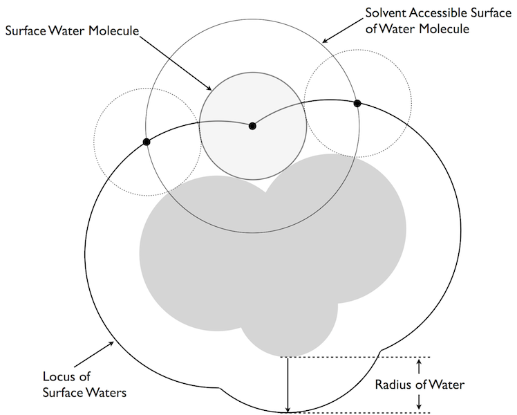
The basic curvature model of Nicholls and Honig [Nicholls-1991].
Unfortunately, Tolman’s formula was only a signpost in that it included a parameter that should be of the order of molecular dimensions but with no clear indications as to what it should actually be. The seminal insight from our work was to associate this parameter with the diameter of water. If this association was made then Tolman’s formula actually described the fractional change of the accessible area of a water molecule at the surface of the droplet, i.e. from \(2 \pi\) steradians at a flat surface to \(4 \pi\) in solution and \(0 \pi\) when isolated from other waters (figure Curvature). The neat thing about this translocation of ideas is that we could calculate a “Tolman”-like correction for any shaped surface, not just a spherical droplet. All we had to do was to put a sphere the size of water (radius 1.4 Ångströms) up to the surface of a molecule and calculate its loss of accessible area. If the surface was planar you lost exactly half its accessible area, if the surface was concave more area was lost and if it was convex less was lost. The idea was very simple: water likes being in contact with water and its own accessible area was a measure of how happy (energetically favorable) it was. As described in our Science paper [Sharp-1991b], this curvature correction became an integral part in our attempt to bridge the microscopic/macroscopic gap. What happened next is, perhaps, an illustration of another gap: that between the simulation world and the continuum world. What was really needed was someone well versed in the simulation world to test the predictions of this model—we had proposed a straight linear correspondence between the loss of area a water might experience and the energy penalty/hydrophobicity at that point in space. Simulations could have at least tested the form of this concept, for instance by simulating water around the surface of an uncharged macromolecule. However, not one simulation group stepped forward because, after all, this is a continuum theory and was seen as competition, at that time, to the simulation approach (and for grant money).
In the end, the majority use of the curvature concept was in graphics; it became a standard way in GRASP to illuminate the convex and concave parts of a protein or DNA. In fact, finding large regions of contiguous concavity proved a useful way to spot areas of functional utility for both. Lost was the concept of this as a quantitative measure of water’s chemical potential.
Then, in 2006, I revisited the problem from a different angle. I’d heard some years ago at an ACS meeting that Alex Rashin, a Russian scientist who had worked with Barry on some of his earliest PB papers, had played around with placing a water, i.e. a molecular representation of water, around a solute and calculating the PB energy of such a water in an attempt to predict, not the total free energy of hydration, but the enthalpy and entropy. This seemed very ambitious and I am not sure if Alex published his results. Barry’s opinion was that perhaps Alex believed a little too much in PB and was pushing the theory too far. However, by that time I was looking at our ability to predict the transfer of small molecules from vacuum to water and it was clear that there were persistent outliers the theory was only just capturing. For instance, tetrafluoromethane has a very unfavorable transfer energy of \(+3.1 \, kcal \, mol^{-1}\), yet PB wants to make this molecule almost soluble (predicts around \(0.0 \, kcal \, mol^{-1}\)). Even if you turned off all the charges in this molecule and just assumed it was a waxy blob you would only get a prediction of about \(+1 \, kcal \, mol^{-1}\). PB just does not have the facility to correctly predict \(+3.1 \, kcal \, mol^{-1}\). Another example, in the opposite direction, is bromoform, i.e. a methane with three bromines attached. In this case the experimental result is \(-1.98 \, kcal \, mol^{-1}\) but PB predicts an unfavorable \(+1 \, kcal \, mol^{-1}\) transfer energy (essentially because there is little polarity in the molecule and it is big and bulky). Now, an all-atom simulationist would look at this and immediately recognize the problem: van der Waals. Fluorine has very small van der Waals interactions and bromine has large ones—using a single area term is bound to fail for these molecules. This may well be a part of the problem, however thinking back to the curvature model I could see another. Fluorinated compounds are often used by the electronic industry where the goal is to reduce the cross-talk between circuits; fluorinated materials have a lower dielectric and hence electrical signals propagate less through them. Similarly, the refractive index of fluorinated compounds is always lower than that of unfluorinated compounds. Bromine (and Iodine) force the dielectric in the other direction, both are more polarizable. Neither observation should be a surprise since VDW interactions themselves are the result of virtual polarization of electron clouds: fluorine is hard to polarize and hence has smaller VDW interactions. Could this effect be captured by PB? Traditionally we think of the solvent as the volume that polarizes in PB, not the solute, but there is nothing to stop us including a solute dielectric to represent its polarizability. This will affect the solvation energy and it does so in the right way, i.e. tetrafluoromethane is less soluble in a polarizable model, bromoform is more soluble. However, it also occurred to me that this will affect the hydrophobic effect as well. If the root of hydrophobicity is that water would rather interact with water than hydrocarbon then surely this will depend on how polarizable that ‘hydrocarbon’ might be. This was the concept I explored before and presented at CUP 8 in February, 2007 and forms, in many ways, the theoretical basis for SZMAP.
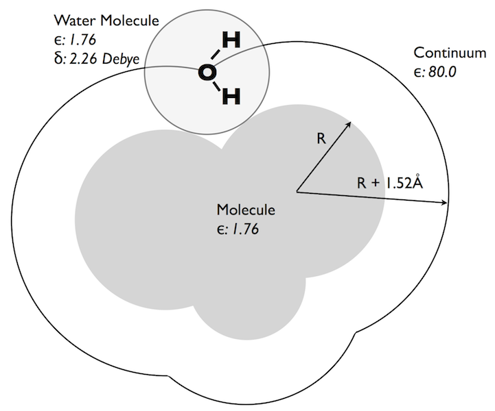
CUP8 Model
Basic physical properties of the CUP8 model for dielectric hydrophobicity. Note: SZMAP currently uses a protein/probe dielectric of 1.0 and the probe water dipole is 1.86 Debye.
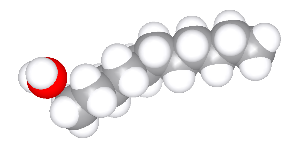
Water Probe
Sampling of contact positions of water against a conformation of a large alkane.
The basic idea behind what I refer to as a Dielectric Theory of Hydrophobicity is illustrated in figures CUP8 Model and Water Probe. Essentially, one does a lot of PB calculations where the only charged molecule is a water molecule pressed up against a solute of interest. The solute ‘desolvates’ water, i.e. produces a small energetic penalty for water at the surface of a solute. Each such water has many orientations possible to it, some of which will be more desolvated than others, e.g. orientations that have protons closer to the solute. If you sample enough orientations then the Boltzmann average of those energies produces a ‘partition function’ for the water ‘partitioning’ from bulk to the surface of the solute. From the partition function you can derive any thermodynamic property you like, e.g. enthalpy or entropy, with one caveat. That caveat is that the energies that make up the partition function are themselves free energies—they are the energies of ‘binding’ a water molecule to the surface of a solute in a particular orientation. They are free energies because that is what PB calculates (essentially, the electrostatic energies in PB are derived from the reorganization of the dielectric, which is a work function, which therefore produces a free energy). As such, each term in the partition function is already a free energy and contains a component of enthalpy and entropy that we cannot separate out. However, we can produce a measure of entropy, i.e. the entropy due to the restriction of orientation of the water (because there are preferred directions of the water up against the solute). We just have to remember that this is not the total entropy of binding/hydrophobicity, because some of that is wrapped up in the PB (free) energy. Similarly, we can calculate an ‘enthalpy’, which is really the average free energy of binding because it is, in fact, the Boltzmann average of the free energy of binding. The free energies are real, the thermodynamic decomposition in SZMAP is incomplete.
What was surprising about the exercise described above is what happens if you use the basic physical properties of water in the model: Bondi radii, dielectrics derived from refractive indices, charges based on vacuum dipoles and typical estimates of water density, i.e. how many waters are likely to cover a solute (figure CUP8 Model). These basic values for water accurately reproduce the transfer of energy from vacuum to water, but surprisingly produce an energetic cost per square Ångström very close to what is seen experimentally, e.g. around \(32 \, cal \, {Angstrom}^{-2} mol^{-1}\). Furthermore, the flat surfaces of molecules like benzene gave higher than expected hydrophobicity, unless the higher polarizability of such was also included, in which case the value fell back into the same range as aliphatic molecules (figure Oil-Water Transfer). For an unparameterized model the result was surprisingly sensible. Furthermore, from vacuum-water surface tension you could predict the non-polar term for the vacuum-water transfer energy term to be right where one would expect, i.e. in the \(6 \, to \, 10 \, cal \, {Angstrom}^{-2} mol^{-1}\) range, except that this value would be dielectric dependent, i.e. lower for polarizable molecules and higher for the unpolarizable. This dependence empirically seems to remove most of the observed variance from experiment seen in the halide containing molecules in the Rizzo set [Rizzo-2006] we have used for vacuum-water transfer energy prediction (figures AM1BCC and AM1BCC+QM Corrected).
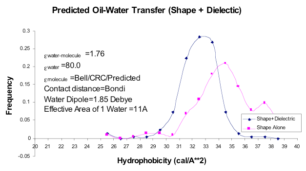
Oil-Water Transfer
The results from the investigation of dielectric hydrophobicity. Using only shape, with no regard to the dielectric constant of the solute, gives the two peaked curve. Including the solute dielectric, which is normally greater than the electronic polarization of water (1.76 relative to vacuum), shifts the curve to smaller values and also brings flat, aromatic molecules into the same distribution as aliphatic molecules. Note: SZMAP currently uses a protein/probe dielectric of 1.0 and the probe water dipole is 1.86 Debye.
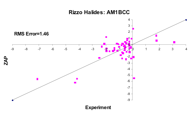
AM1BCC
The subset of molecules from the Rizzo set containing F, Cl, Br or I, using AM1BCC charges with Bondi radii.
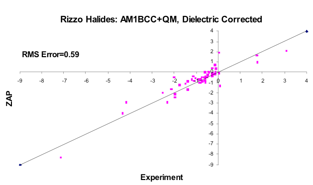
AM1BCC+QM Corrected
The subset of molecules from the Rizzo set containing F, Cl, Br or I, using better quality charges (correcting the AM1BCC parameter for Iodine, for example) and the dielectric version of hydrophobicity outlined here.
Hydrophobicity vs Curvature
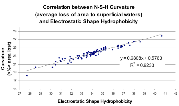
Correlation between the net curvature of ~100 small molecules from the Rizzo set and the *SZMAP-type energy function (molecules uncharged). Note that curvature here is represented as % of area lost, i.e. more area lost means more energy to place a water molecule in this position.*
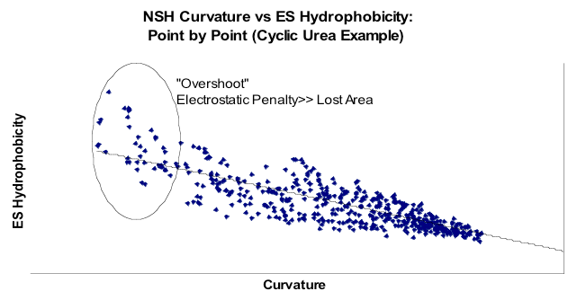
Finally, how did this explicit enumeration of orientations and positions compare to the very simple Nicholls/Honig curvature model from 1991? Figure Hydrophobicity vs Curvature illustrates that there was a strong correspondence when both curvature and partition function were averaged over the entire surface of a subset of small molecules from the Rizzo set [Rizzo-2006]. More interesting was to look at the point by point comparison of the free energy approach and curvature. This is shown in figure Curvature vs Hydrophobicity. What this shows is that there is good correlation between the two models when the curvature is small, but that when the curvature is large, i.e. a water begins to be enclosed by the solute, this agreement breaks down, i.e. it takes more energy to bury a water than it does to merely make it sit on the surface of a convex solute. The reason this was good news is that the attempt to bridge the microscopic/macroscopic gap in 1991 had had to rely on other factors than just curvature because the effect was just not big enough. Here the results suggest why, i.e. that planar surfaces are more hydrophobic than the simple curvature model predicts. In fact, by constructing a planar surface from methyl groups the CUP8 procedure gets close to the macroscopic value (\(62 \, cal \, {Angstrom}^{-2} mol^{-1}\)).
Curvature vs Hydrophobicity
Correlation over the surface of a single molecule, a cyclic urea. Note that in this graph curvature is as traditionally defined, i.e. larger means more convex, i.e. less area occluded. Note, therefore that in regions of most negative curvature the non-polar term from ZAP increases above the trend line.
All of this leads to SZMAP because the next step in this work is to allow the solute to be charged, i.e. to introduce possibly compensating effects for a surface water due to the electrostatic field produced by the solute. For instance, the interactions between a water and a charged group will be favorable and will overcome the desolvation of the water, relative to the rest of the bulk solvent. And this is essentially what SZMAP attempts to estimate, i.e. it is the exact same procedure of estimating the binding energy of water over a set of orientations. In the initial version of SZMAP a discrete set of orientations are used, however there are ways in future versions for this to be made more comprehensive, with little loss in speed. The other change we introduce is to allow the sampling of water positions that do not make contact with the solute. The reason to do such was brought home to me during conversations with Eric Manas of GSK. He pointed out that the model should suggest water would begin to lose contact with other water before it actually touched the surface. In fact, based on close packing arguments the distance two surfaces would have to come before there was an effective surface-surface force due to dewetting would be \(Diameter_{water} + \sqrt{3 \, Diameter_{water}}\), i.e. about 6 Ångströms—close to that seen by simulations by the Berne group at Columbia [Huang-2003]. As such, SZMAP calculates a volume function, not a surface function such as the curvature function in GRASP. Of course, this may also mean that the concordance between experimental alkane-water hydrophobic energies and the CUP8 work was partly fortuitous, i.e. there would more formally be energetic contributions from positions further way from the surface.
The remaining difference in SZMAP is that we decided to take on the VDW interaction of water to the solute, namely by adding the VDW energy for each orientation of the water to the solute. We felt this was important for a couple of reasons. For one thing we know it will move the desolvation energy in the correct direction for polarizable atoms. We also can prevent anomalous interactions, e.g. close contacts between protons and charged groups that would be compensated for by VDW repulsion. Finally, in PBSA theory we have the choice of either using a buried area term (typically \(25 \, cal \, {Angstrom}^{-2} mol^{-1}\)) or explicitly calculating the VDW interactions and using a much smaller area term (for instance \(6 \, cal \, {Angstrom}^{-2} mol^{-1}\) when using AM1BCC charges). As we are aiming at some verisimilitude with reality it seems a straightforward choice to explicitly include VDW. As a consequence, there should be a small residual area term that depends on the buried accessible area of the water.
A few words on how points are chosen. We use the shape scoring function in FRED to provide positions of water that are making some contact with the protein, removing points that VDW would clearly disallow [McGann-2003]. This provides a regular lattice of points on which the oxygen of water is positioned. The orientations are calculated for the protons about this center. One of the advantages of using PB technology for this process is that for each water orientation we get a potential field throughout the protein. This field can be used to calculate interactions with many different protein charge states. We have not implemented this at present, but it will be a feature in future versions of SZMAP.
At present the output from SZMAP consists of the thermodynamic quantities calculated at each grid point, i.e. the rotationally averaged free energy of a water in each position. The breakdown that we can do into entropic and enthalpic contributions is included, as are the classic curvature values. From our previous work we anticipate these volume functions will yield interesting and quantitative numbers, for instance the energy of displacing water, whether relative or absolute, and the prediction of ‘condensed’ water, i.e. what are typically, but incorrectly, referred to as crystallographic waters. Most such labeled waters are figments of crystallographer’s desires to reduce their R factor, but some are real, i.e. some waters are undoubtedly bound substrates to the protein. It may also be possible to build chains of water from the preferred orientations and positions of single waters, although the thermodynamics and physics of this process are more dubious. We can also include more polarization physics, for instance by implementing the EPIC model of Jean-Francois Truchon [Truchon-2009]. At this point SZMAP is a tool, an engine for discovery.
Anthony Nicholls, Santa Fe, 2010.