Technical Details
Energy Calculations
Energy values are calculated at each grid point as follows. The energy for each probe water orientation j is the sum of the ZAP protein:water Coulombic interaction energy, the protein and water desolvation penalties and the van der Waals energy. For speed, the protein desolvation term is not computed for each orientation, but is instead computed once per grid point using a spherical united-atom representation of the probe water.
The partition function Q is the usual sum:
The probability of each orientation is then:
The probe water orientation entropy difference from continuum water is:
Likewise, the probe water free energy difference from continuum water is:
And of course, the enthalpy difference is the sum:
The variance in estimated energies varies with the number of random probe orientations sampled. See figure Variation in Energy Estimates. At 50 random orientations per point, half of repeated free energy estimates are within about \(0.2 \, kcal \, mol^{-1}\) of one another. This gives us a way to examine the balance between precision and calculation speed. Symmetrical probe orientations, the default in SZMAP, are completely reproducible and sample positions evenly. Sixty symmetrical orientations produce reliable energy estimates, but when more precision is required, 360 symmetrical orientations are recommended.
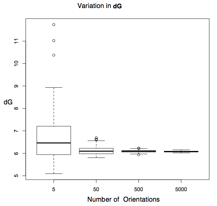
Variation in Energy Estimates
Box plots for repeated calculations of free energy at a single point using random orientations. The mode is indicated with a heavy line, rectangles enclose 50% of data points and the whiskers enclose 90%.
The probe water order parameter represents the fractional loss of entropy due to electrostatics:
where \(prob^*_j\) is the probability for orientation j based on the electrostatic energy terms only, without the van der Waals term. Order calculated in this way is highly correlated with the neutral difference entropy.
Water Geometry, Radii, and Charges
PB calculations require you to know three things for each atom: the position, the charges and the radii. What should we use for water? The geometry for the probe water in SZMAP is the same as for “TIP” water: \(r(OH) = 0.9572\) Å and \(HOH \, angle = 104.52^{\circ}\). Work for SAMPL meetings has shown that Bondi radii are a good starting point for PB calculations, although some atoms tend to need slight adjustments, for instance carbonyl oxygens always seem to want to be slightly bigger, nitrogens smaller. Water is an odd case as no other oxygen behaves chemically in the same way. So by the principle of maximum indifference we just use Bondi radii (H: 1.20 Å and O: 1.52 Å).
What charges should we use? Most force-field charges give water a dipole of between 2.4 and 3.0 Debye. This might seem odd because the actual, vacuum dipole of water is 1.86D. The force field community justify this because water is polarized in solution with estimates of its polarized dipole in the range of that used in force-fields. It is typical of this community—charges are over polarized to attempt to account for the lack of polarization in their models. AM1BCC, for instance, gives water a dipole of 2.24D, about 20% too large. This has consequences for the vacuum-water transfer energy—PB predicts an electrostatic component of transfer for AM1BCC charges and Bondi radii of \(-9.95 \, kcal \, mol^{-1}\). Add to that a typical “hydrophobic” term (yes, for water!) of about \(+0.65 \, kcal \, mol^{-1}\) (surface area of \(107 \, {Angstrom}^2\); \(6 \, cal \, {Angstrom}^{-2} mol^{-1}\)) this gives us \(-9.3 \, kcal \, mol^{-1}\) prediction for vacuum-water. The only problem is that the experimental value is about \(-6.3 \, kcal \, mol^{-1}\). This is a huge % error for a simple model and would be very bad news for SZMAP since we want to estimate the energy of a water molecule burying itself into an active site. What happens if instead we use charges that reproduce the vacuum dipole? The electrostatic component becomes \(-6.9 \, kcal \, mol^{-1}\). Adding the ubiquitous surface term we get \(-6.25 \, kcal \, mol^{-1}\), i.e. just right. But what about polarization? Well, we are using protein charges that are also derived from vacuum potentials so in some ways this is not an inconsistent description. Overall, at this stage we feel it is more important to correctly calculate the desolvation of water. Therefore SZMAP uses point charges for hydrogen and oxygen of +0.327 and -0.654, respectively.
The next stage may be to use a simple polarization model presented at CUP7 that involved a real molecular dielectric (i.e. \(\epsilon = 2\)) and an increased radius for each atom. In this model water would have charges with a dipole of 2.48D in line with experimental estimates. Preliminary results from this model suggest that for many situations the binding energies of molecules is not dissimilar from unpolarized models. A further step will be to use the EPIC model developed by Jean-Francois Truchon at Merck-Frosst [Truchon-2009].
Uncharged Water, Difference Energies, Bubbles, and Stabilization
The values SZMAP calculates for \(\Delta G\), \(\Delta H\) and \(T \Delta S\) represent differences between the explicit probe water and the continuum water. In other words, a positive \(\Delta G\) indicates that the continuum model over-estimates the cost of displacing water at that position. When trying to decide which modifications are most likely to increase binding affinity, we would prefer to compare the water probe to the ligand atom that displaces it, or at least a proxy for the ligand atom. In SZMAP, this proxy is the water probe without any of the energy terms that involve a charge on the water (leaving only \(P_{desolv} + VDW\)). Because these energy terms have already been determined, calculating the properties for this “uncharged” or “neutral” water requires no additional time, it’s free. The difference in free energy between standard and uncharged water is negative where standard water is more favored and positive where the uncharged water, our hydrophobic group proxy, is more favored.
SZMAP can also calculate the difference between our probe and a vacuum bubble of the same size (defined as just the \(P_{desolv}\) term). Because protein desolvation is treated as constant over all probe orientations only the vacuum free energy and enthalpy differences are calculated, not the entropy differences.
Grids are masked such that regions where the sum of the van der Waals and interaction energies is greater than a cutoff (by default \(0 \, kcal \, mol^{-1}\)) are set to zero. This is done so that grids are displayed only in regions where solvent atoms can physically fit.
As to how to interpret these difference grids, it should be beneficial for a hydrophobic ligand atom to overlap a region where the neutral free energy difference is positive because this involves displacing water that is less favorable than the neutral probe. Overlapping a region where the neutral free energy difference is negative, on the other hand, requires the overlapping group to be at least as polar as water and making a similar level of interactions.
Finally, SZMAP can calculate stabilization energies from the neutral difference values as a reaction energy
where bulk-solvent is defined as \(0 \, kcal \, mol^{-1}\).
Negative free energy values indicate water is stabilized at that location in the complex, over and above the same location in the ligand and the apo pocket. Positive values are found where the water is destabilized in the complex. The stabilization or destabilization says nothing about the actual level of stability, so these energies need to be compared to others such as the apo or complex neutral difference free energy.