Example Commands

This section has several examples of typical SZYBKI command-line executions.

Protein preparation

X-ray protein structures rarely contain all hydrogen atoms coordinates. It is necessary therefore to prepare the protein structure before any protein-bound ligand calculations are done.

prompt> szybki -optGeometry Honly -prefix ex1 -neglect_frozen protein.pdb proteinH.mol2

In this command the input protein file protein.pdb is assumed to contain all heavy atoms. Option -optGeometry followed by the string Honly fixes all heavy atoms at their positions given in the input file. For larger proteins it is recommended to increase the total number of optimizer iterations beyond the default value of 1000 using the option -max_iter. It might be particularly important if a tight convergence of 1e-6 or smaller is required (see -grad_conv). The output protein file is proteinH.mol2. Note: All ionizable residues are assumed to be in their standard ionization states. If other than standard ionization states are needed, the input file has to be edited accordingly before the SZYBKI run is done.

Ligand optimization in solution

The equilibrium geometry of a molecule in solution is sometimes drastically different than in vacuum. This is because of solvent forces. The most efficient way to optimize a large set of ligands in solution is the usage of the -sheffield option.

prompt> szybki -sheffield -am1bcc -prefix ex2 ligands.sdf ligands_optimized.sdf

In the run above, a set of molecules from the input file ligands.sdf is optimized with the MMFF94 force field in solution. AM1BCC charges are optionally used for the Sheffield solvation model. Skipping the -am1bcc would result in the usage of MMFF94 atomic charges. Optimized structures are written to the ligands_optimized.sdf file. One can also optimize the ligand in solution using a physically more rigorous model by solving the Poisson-Boltzmann equation at every step. The command line below is equivalent to using the widely known PBSA model:

prompt> szybki -solvent` ``PB`` -solventCA 0.005 -prefix ex3 ligands.sdf ligands_optimizedPB.sdf

Optimization with fixed atoms

This example illustrates the usage of the option -fix_file.

prompt> szybki -fix_file f.txt -prefix ex4 mymolecule.mol2 molecule_opt.sdf

Text file f.txt contains molecules names followed by atom numbers in the (0,1…N-1) numbering convention. For example the f.txt file contains the following 6 lines:

Molecule1

0

15

Molecule2

5

9

informs SZYBKI that atom 0 and 15 for molecule Molecule1 and atoms 5 and 21 for molecule Molecule2 should be fixed during optimization. This flag is useful when the user wants to fix atoms which are not directly bonded, for example they belong to different functional groups in the optimized molecule. In the case a common substructure has to be fixed, an option -fix_smarts is more convenient to use:

prompt> szybki -fix_smarts fix_smarts.txt -prefix ex4a mymolecule.mol2 molecule_opt1.sdf

where file fix_smarts.txt contains a single line with the SMARTS pattern c1ccccc1 which defines the substructure to be fixed.

Ligand entropy calculation in solution

Assuming that the molecule conformations are given in the molecule.oeb file, the command line execution:

prompt> szybki -entropy AN -sheffield -prefix ex8  molecule.oeb

will result in the standard molar entropy estimation of the input molecule in solution. The meaning of the parameter value AN is explained in the description of the option -entropy. Option -sheffield informs SZYBKI that the calculation will be done in solution with the use of the Sheffield Solvation Model. The entropy results will be written in the ex8.log file. If the input file molecule.oeb does not contain the complete ensemble of conformations, the resultant entropy value may not be accurate. We recommend therefore that the input conformations are generated with the OpenEye tool OMEGA, with the omega -rms option set at 0.1 value, and omega -maxconfs set to at least 1000.

Protein-bound Ligand entropy calculation

Run:

prompt> szybki -p protein.mol2 -entropy AN -prefix ex9 ligand.mol2

will generate the estimation of ligand entropy in the active site of the protein. Input file ligand.mol2 might be a docked structure or preferentially the X-ray structure.

Binding entropy calculation

A workflow for estimating binding entropy is shown in the figure below:

Binding Entropy Estimation

A basic workflow for binding entropy estimation.

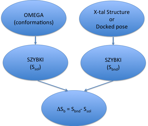
As Figure 4.1 shows, estimating binding entropy, \(\Delta S_b\), requires two separate SZYBKI runs: one for the estimation of ligand entropy in solution (\(S_{sol}\)) and another one which calculates protein-bound ligand entropy (\(S_{bnd}\)). It is possible to calculate binding entropy (\(\Delta S_b\)) in a single SZYBKI run:

prompt> szybki -complex complex.oeb -entropy AN  -prefix ex10 -sheffield -in ligand.oeb

where complex.oeb is a molecular file of the protein-ligand complex and ligand.oeb contains an ensemble of conformations of the ligand in solution. Note: The docked ligand in the complex.oeb file must represent a single pose and must be the same molecule as in the ligand.oeb input file. In the case where two or more docked poses are used, calculation of binding entropy requires two separate runs as shown on Figure 4.1.