The WaterColor extension is used to set-up SZMAP
and GamePlan output in VIDA.
For SZMAP grids, it alters the contour surface display properties.
It sets up a standard color scheme for grids, sets some grids to solid surfaces
while leaving others wire-mesh,
sets up any difference grids to show both positive (yellow) and negative (purple) contours,
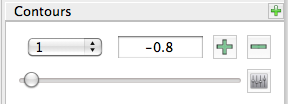
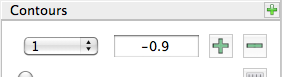
and sets the contour levels to “reasonable” default values. Feel free to change any of
the properties afterwards.
It also restricts the display of protein atoms to just those that surround the ligand
and turns on the display of both the protein and the ligand. And protein molecular surface
is added to the protein, but not displayed by default.
For GamePlan results, the extension makes the annotation visible. It also
restricts the protein and ligand display and generates a molecular surface as described for grids.
This extension is not required to analyze -at_coords results but if engaged,
will set the protein and ligand display as above, along with the molecular surface.
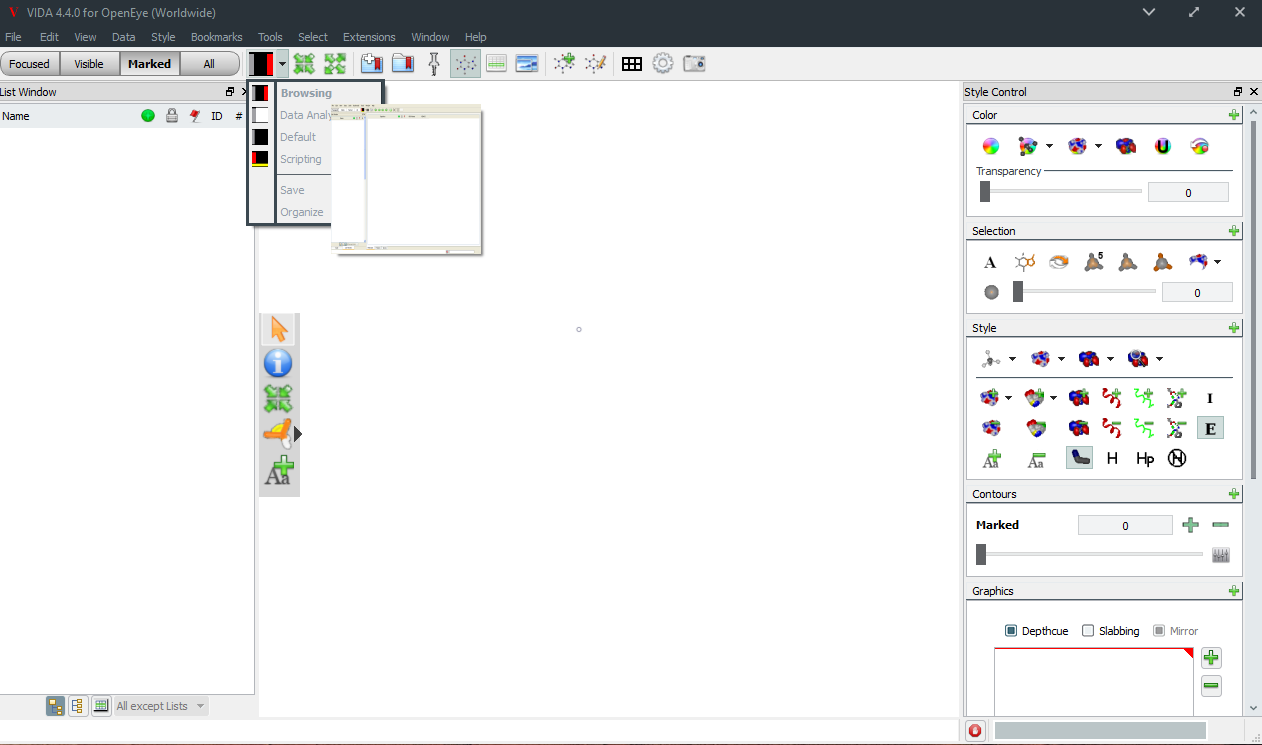
Open VIDA and make sure the 3D viewer, the list panel
and the style panel are available. If not, select the Browsing view
(figure Browse View) to setup your display.
You can move the list and style panels to as needed—here, we
have stacked them on top of one another to save space.
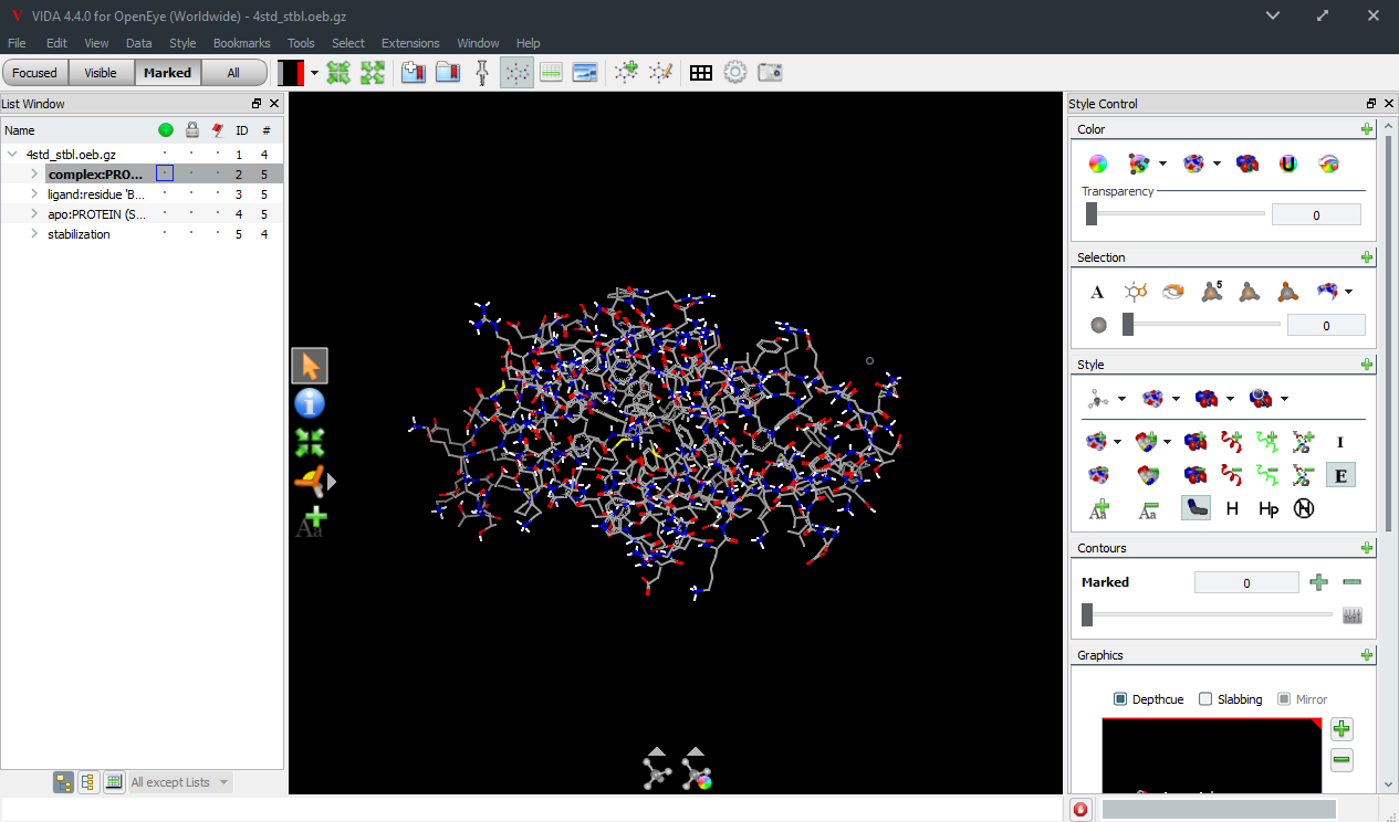
Select File >> Open and choose the .oeb.gz or .oeb file containing
your SZMAP grid results.
The file should show up in the List Panel
and the structure should show in the 3D viewer.
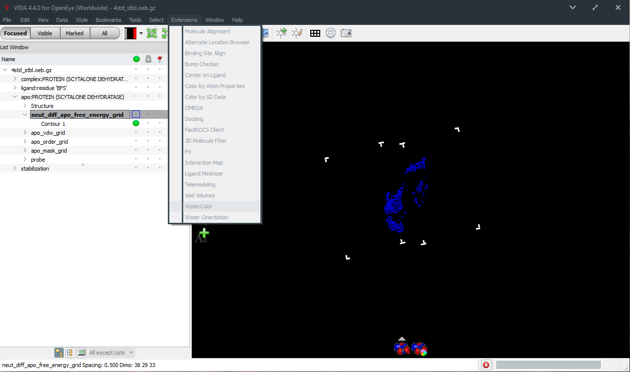
Run the WaterColor extension
(figure WaterColor Extension),
to set the contour levels to better
starting values and also change the colors and
rendering styles so that the various grids are
easily distinguish.
These settings can be modified using the style panel.
It also hides all protein atoms that are not near to the
binding site.
Finally, it generates a molecular surface associated with the protein
that shows the boundary of the binding
site. This surface can be selected and displayed in the same way as a grid.
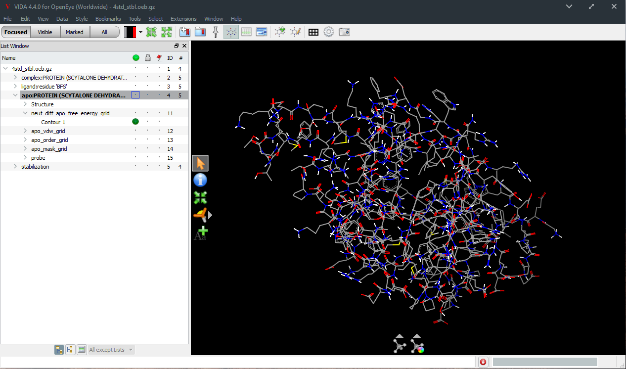
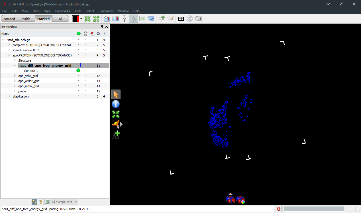
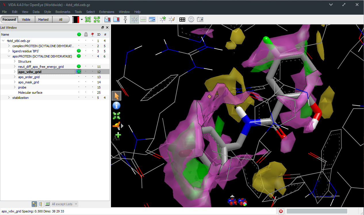
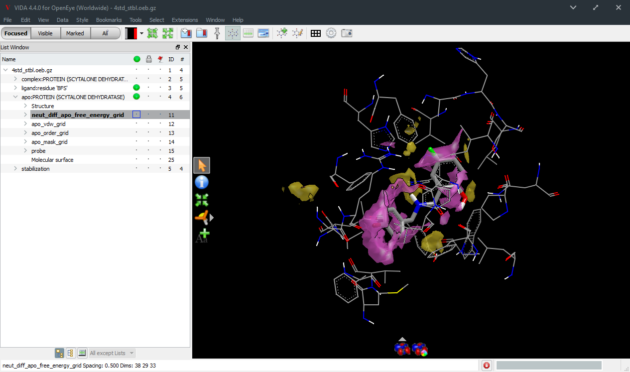
After WaterColor runs, the ligand and protein should have a green dot in the visibility column.
If it is not visible, click on the neut_diff_apo_free_energy list item to show
that grid in the context of the input molecules
(figure Molecule and Grid).
Step 6
The scene can be scaled (or zoomed) by holding down the
Middle mouse button by itself, the Left and Right mouse
buttons together, or by using the mouse wheel. The scene can
also be scaled using the W and S keys on the keyboard.
You can change the color of the grid and switch between wireframe
lines, solid surface, and point clouds (select the ^ button above the surface
icon at the bottom of the 3D display
figure Surface Style;
points have jitter added).
Overlapping contours from different grids requires that you select
all the grids in the list panel (figure Multiple Grids).
This can be a little counter-intuitive;
play with multiple selections until you get the hang of it.
Hint
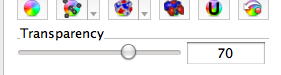
Only select one grid at a time if you are trying to change
the color or style or transparency to a value different
from other grids.
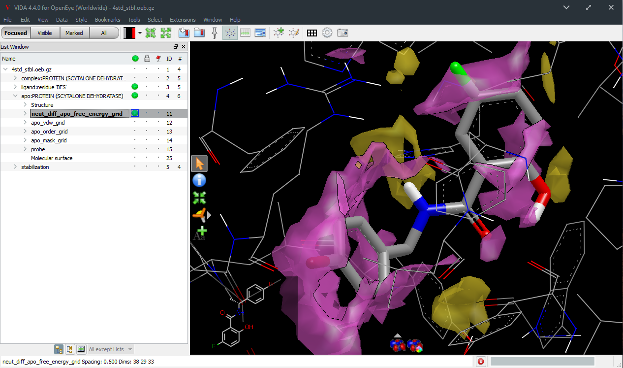
Difference grids represent the difference between standard water
and uncharged water, a proxy for hydrophobic atoms in the ligand.
The WaterColor extension configures them as
a pair of contours: negative in yellow representing
areas where standard water has lower values—for \(\Delta G\)
and \(\Delta H\)
standard water is more favorable here—and positive in purple
representing areas where uncharged water has lower values
(figure Difference Grid).
The hydrophobic/hydrophilic pattern within a site is matched
by high-affinity ligands.
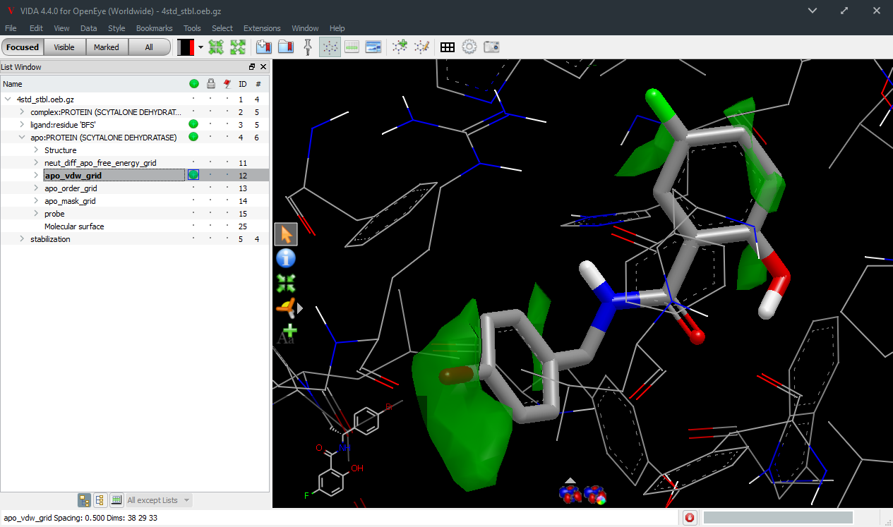
Van der Waals grids show a component of the energy
that is not a part of the difference free energy (because it subtracts out).
The default VDW (green) contours are -2 kcal/mol, containing the lowest 5% (approx.)
of the negative VDW waters (figure VDW Grid). Low VDW regions
are found in regions with weak polar interactions. Conversely, regions with
strong polar interactions have positive VDW energy. The balance between
Coulombic interactions and VDW interactions defines the masked, or nonclashing,
region.
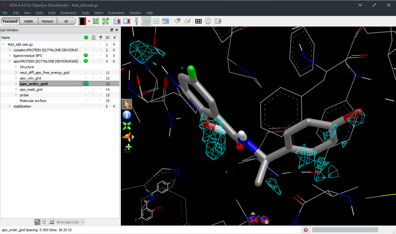
Order grids (light blue mesh) show the fraction of water entropy lost due to electrostatic
interactions (figure Order Grid).
A value of 1.0 means the site is highly ordered and displacing water from there will
liberate almost all this rotational entropy (approximately 2.4 kcal/mol). A value of 0.0 means
the water orientation is completely degenerate and displacing it will not liberate any
rotational entropy. The energy gained by displacing water is primarily entropic,
enthalpy mainly serves as a filter that discriminates between different ligands.
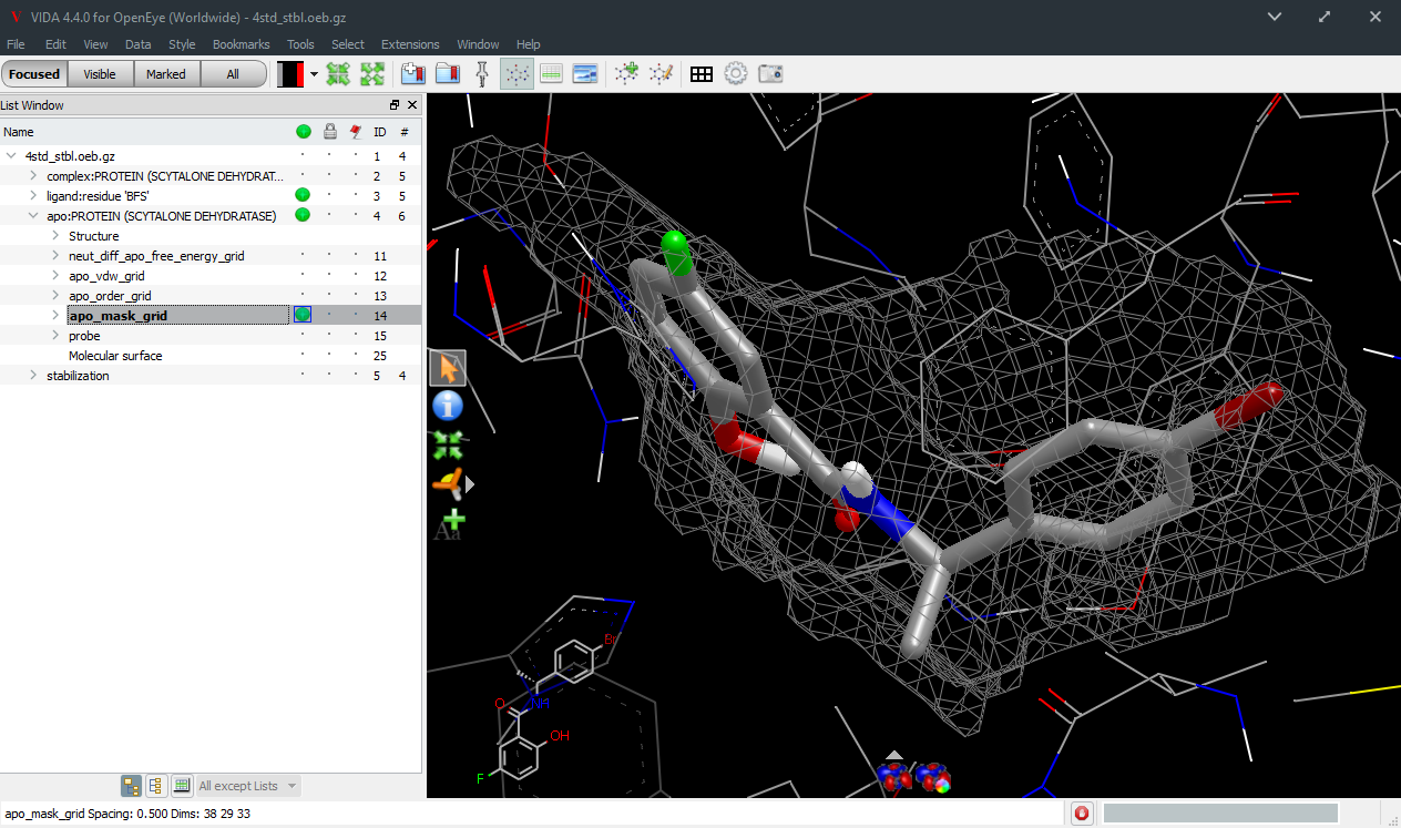
Mask grids (gray mesh) are an accurate description of the solvent accessible surface,
calculated as regions where the minimum Coulombic interaction + VDW energy is below a threshold
(figure Mask Grid). Examining the mask grid clarifies where water
fits and where it clashes. The displaced region of the apo pocket contains the volume
of the apo mask minus that of the complex mask. To speed up ligand calculations
during a stabilization run, the ligand analysis is limited to the region within
the complex mask, by default. In “at_coords” calculations, points that are not
in the mask are labeled “CLASH”.
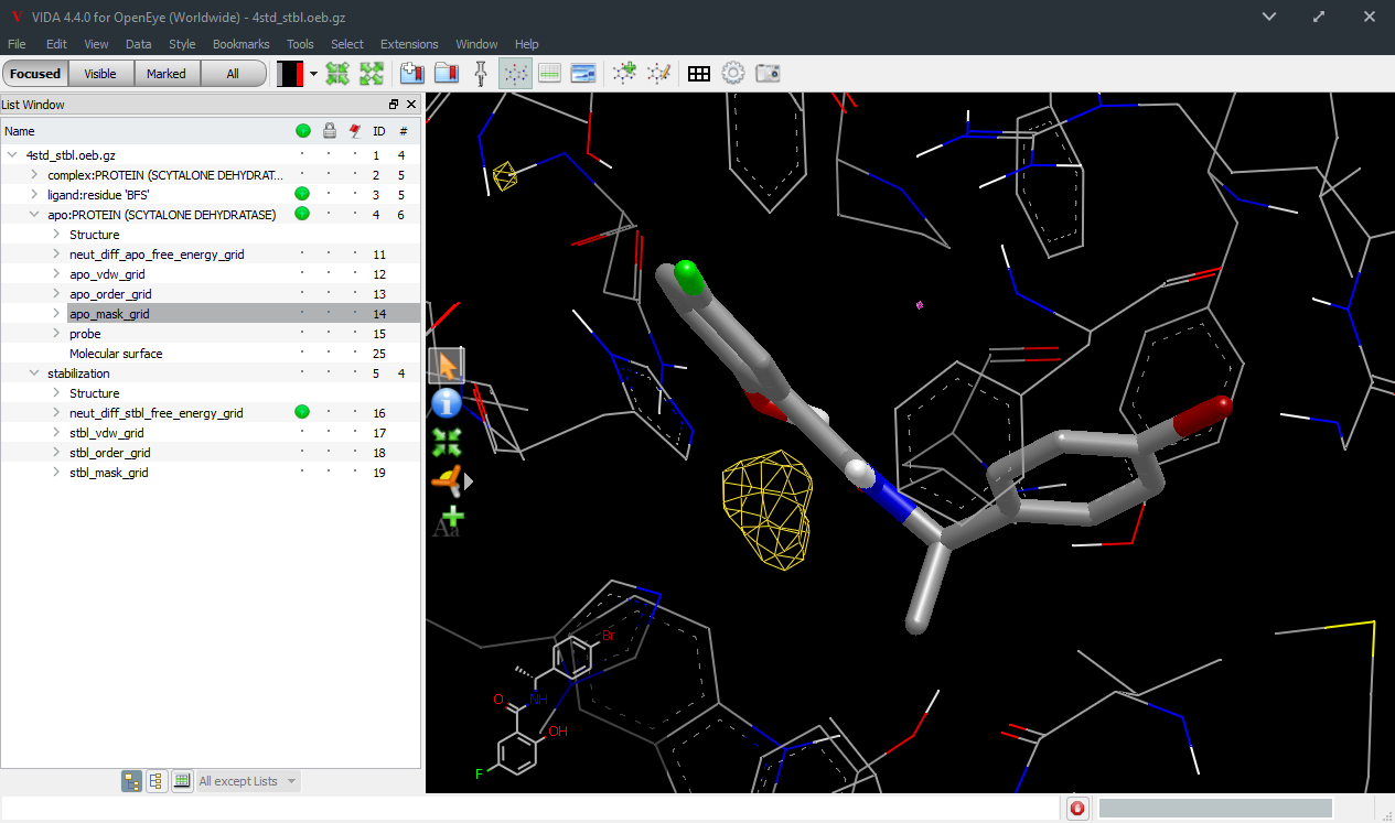
Stabilization grids
are special kinds of difference grids (complex - apo - ligand),
showing how water is stabilized
or destabilized upon binding (figure Stabilization Grid).
They provide information about the possible
effects of modifying the ligand.
If you have calculated displacement grids—with apo data in regions where water has
been displaced—these will be found at the end of the list of items in the results.
Examining them can clarify how far a ligand’s reach extends.
Other grids can be produced but these capture the main elements required to understand solvation.
Open VIDA and make sure the 3D viewer, the list panel
and the style panel are available. If not, select the Browsing view
(figure Browse View) to setup your display.
Select File >> Open and choose the .oeb.gz or .oeb file
containing your GamePlan results.
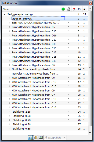
The file should show up in the list panel
(figure Gameplan List Window;
the blue bar identifies the active entry)
and the ligand structure should show in the 3D viewer.
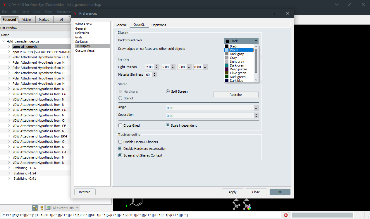
The figures shown here have a white background which is recommended for
presentations and publications. You can change the background color in
VIDA by bringing up the Edit >> Preferences window
(Vida >> Preferences on Mac OS X),
selecting 3D Display and then clicking on the OpenGL tab
(figure Changing Background).
Step 3
Run the WaterColor extension to activate the display of annotation
explaining the various ligand modification hypotheses.
It also adds a surface that shows the boundary of the binding
site, and hides all protein atoms that are not near to the
binding site. These settings can be modified using the style
panel.
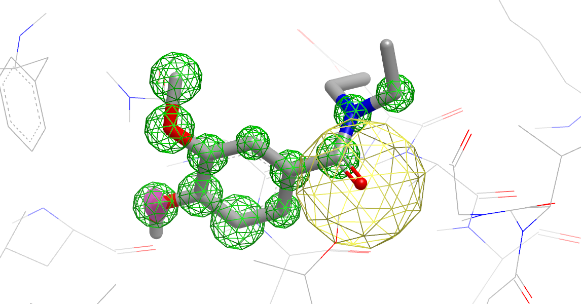
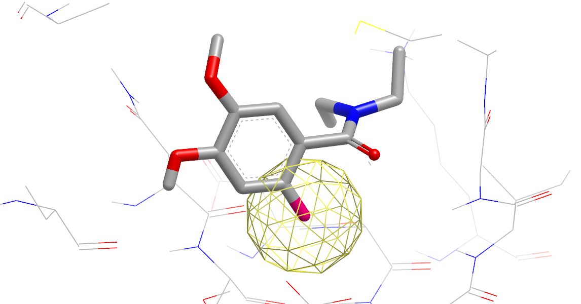
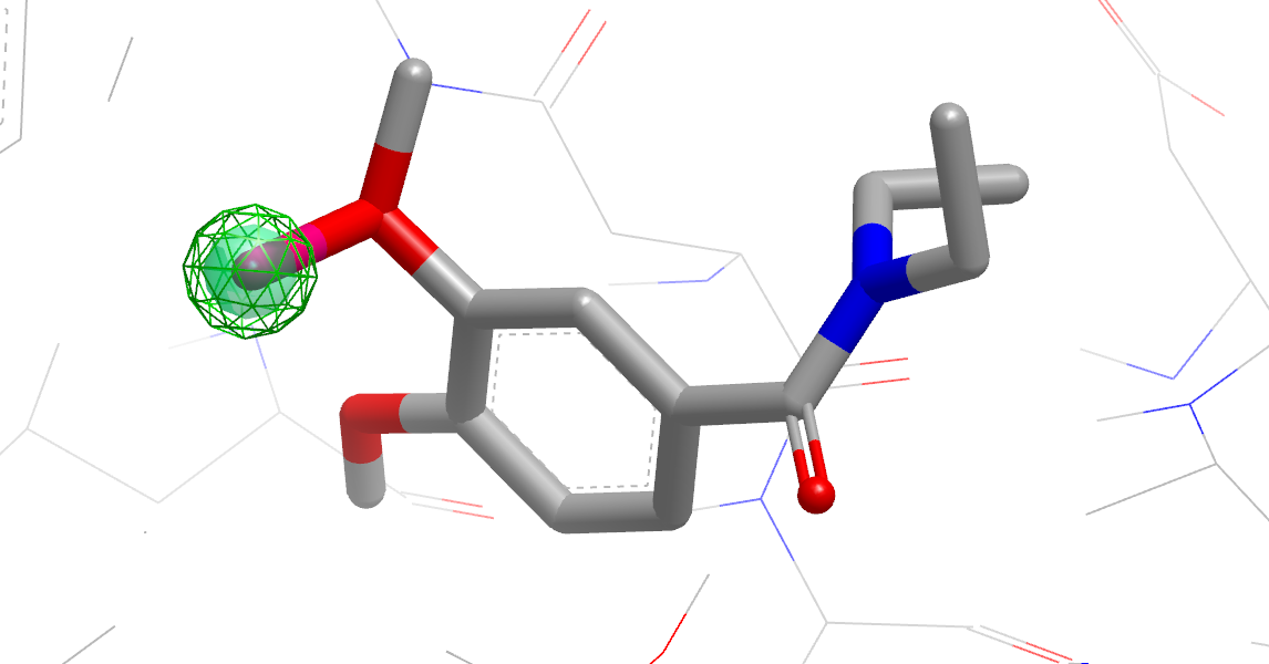
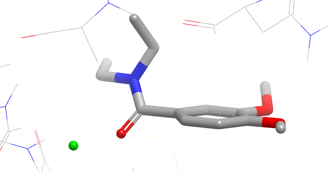
The first entry analyzes how the ligand
(figure Ligand Compared to apo Binding Site)
Yellow mesh spheres show polar sites, green mesh spheres are van der Waals sites,
translucent green spheres are non-polar sites, and purple diamonds indicate
a mismatch, where the ligand is either much more or much less polar than the binding site.
See chapter GamePlan for a complete description of the
annotation symbols.
Next comes the apo-protein, then a series of
hypotheses for ligand modification.
Scarlet colored bonds indicate a proposed modification
to the ligand. Gameplan tries to explore a wide
range of possible ways to improve the ligand, and has an
option that permits the hybridization to differ from
that in the original ligand. See the
-sample_hybridization option in chapter GamePlan
for details.
Using the arrow keys to step between the different
hypotheses, you will
see yellow cages around atoms where water makes good polar
interactions (figure Hypothesis for a Polar Substituent),
green cages around atoms
where water has good van der Waals energy,
and translucent green balls around atoms
where a fluorine or methyl group may be a good fit
(figure Hypothesis for a Nonpolar/VDW Substituent).
The same substituent may show up with different
conformations or under different categories.
Finally points where
water is stabilizing (green) or destabilizing (red) the complex are enumerated
(figure Stabilizing Site).
Destabilizing points may be good candidates for displacement, while
stabilizing points can be left in place. But if a stabilizing site
contains highly ordered water in the complex, careful replacement
of this water with a substituent that makes the same number of interactions
can liberate as much as 2 kcal/mol of rotational entropy.